User:Epipelagic/sandbox/current1

RESOURCES AND WORKING DRAFTS ONLY

Viruses in the ocean conveyor belt

Viruses shape marine ecosystems by controlling their host abundance and diversity through cell lysis and generate and maintain diversity through horizontal gene transfer (Angly et al., 2006; Rohwer and Thurber, 2009; Zeng and Chisholm, 2012). Moreover, viral lysis influences oceanic productivity by promoting organic matter and nutrient cycling through the release of intracellular material from the host cells (Middelboe et al., 1996; Middelboe and Lyck, 2002).

Several parameters affect the distribution of viruses in the marine environment (De Corte et al., 2012, 2016; Brum et al., 2015). The presence of a suitable host is key to perpetuate the viral “life cycle.” However, other variables, such as temperature (Parada et al., 2007), UV radiation (Wommack et al., 1996) and salinity (Kukkaro and Bamford, 2009), influence the time span that viruses remain active in the ambient water and capable of infecting a host. The effects of these biotic and abiotic factors have been studied in surface waters (Bongiorni et al., 2005; De Corte et al., 2011) and, infrequently, in the deep ocean, where low temperature leads to relatively slower virus decay rates than in surface waters (Parada et al., 2007). The longer bacterial generation time and slower viral decay rates in the deep ocean (Parada et al., 2007; De Corte et al., 2012), together with the limited vertical mixing of the deep-water masses, suggest that oceanic currents and the thermohaline circulation may play an important role in influencing the global distribution of viruses and their hosts (McGillicuddy et al., 2007; Sintes et al., 2013, 2015; Sul et al., 2013; Brum et al., 2015; Frank et al., 2016).

The global overturning circulation (Figure 1) is a system of oceanic currents driven by wind, density and mixing processes (Schmittner et al., 2007; Talley, 2013). The North Atlantic Deep Water (NADW) is formed in the North Atlantic Ocean through the sinking of cold and dense waters, and moves southward toward the Southern Ocean (Talley, 2013). The second limb of the deep overturning circulation system is the Antarctic Bottom Water (AABW). The AABW is formed in the Southern Ocean via mixing of NADW, Indian Deep Water, Pacific Deep Water, and shelf waters originating from Antarctic shelf systems (Talley, 2013).

Viruses, as part of the dissolved organic matter pool (DOM; operationally defined as the organic matter that passes through a 0.2 μm filter), should behave conservatively and reflect the different formation sites of the deep waters (Bercovici and Hansell, 2016). However, it is important to note that certain local effects, such as particle export and in situ production (Nagata et al., 2000; Hansell and Ducklow, 2003; Yokokawa et al., 2013), play an important role in determining bacterial and viral abundance and community composition. Sinking particles provide a source of fresh substrate for microbes in the deep sea (Cho and Azam, 1988; Karl et al., 1988; Follett et al., 2014). Hence, this organic matter might be especially important in the Pacific Deep Water of the North Pacific with its low DOM concentration (Hansell, 2013).

DNA viruses lack conserved marker genes, hindering the assessment of their biogeographical patterns. The dispersal of viruses across the oceans has only been recently explored (Angly et al., 2006; Hurwitz and Sullivan, 2013; Martinez-Hernandez et al., 2017; Gregory et al., 2019). Moreover, most studies addressing viral community composition are limited to the upper ocean layers (Angly et al., 2006; Brum et al., 2015; Hurwitz et al., 2015). Due to methodological limitations, virus-host interactions in the dark ocean have mainly been assessed by microbial and viral enumeration (De Corte et al., 2012; Wigington et al., 2016; Lara et al., 2017). Therefore, little is known about the changes of viral communities along the deep ocean conveyor belt circulation system.

Although viromics (metagenomics of viral communities) is increasingly used to study viral diversity and function in the marine ecosystems (Breitbart et al., 2004; Breitbart and Rohwer, 2005; Hurwitz and Sullivan, 2013; Brum et al., 2015), it has its limitations. Viromics typically requires a large sample volume, which may limit the number of samples that can be collected and processed in a timely manner. Moreover, filtration of water samples to physically separate the viral fraction from other microorganisms may lead to the loss of a fraction of the viral community, in particular of giant viruses, while some small bacteria might pass through the filter (Martinez Martinez et al., 2014).

Microbial biogeochemical roles and ecosystem functioning

The assembly of microbial communities is governed by a joint effect of deterministic (niche) and stochastic (neutral) processes. Subdivision of a microbial community (according to abundance, activity, function and occupancy) into subcommunities will facilitate an accurate view of microbial assembling processes.

Phylogeny and functional traits

To better understand microbial ecosystem functioning, creating links between an individual taxon and a specific function is required. However, it is infeasible to trace all the diverse biogeochemical processes and to relate them to taxa. This problem may be solved from the point of view of the microorganisms, as microbial functional capabilities have been found to connect strongly with phylogeny (Martiny et al. 2013; Zimmerman et al. 2013). For example, the presence of functional genes related to oxygenic photosynthesis, methane oxidation and sulfate reduction has been found to be highly phylogenetically conserved (Martiny et al. 2013). In coastal seawater, recent studies have shown that microorganisms that assimilated organic matter, including starch and glucose, were phylogenetically clustered (Bryson et al. 2017; Mayali and Weber 2018), reflecting phylogenetically conserved resource partitioning in the coastal microbial loop (Bryson et al. 2017). Such phylogenetic conservation in substrate utilization supports similar distribution patterns (even at a broader taxonomic level; Philippot et al. 2010; Schmidt et al. 2016) and similar lifestyles among microbial relatives. Salazar et al. (2015) found that the particle-associated and free-living populations in the deep ocean had different phylogenetic origins. These observations enhance the possibility of inferring microbial functional traits with phylogenetic information.

However, growing evidence now suggests that variations in functional traits occur within closely related microbes, even at the loosely defined species level (Larkin and Martiny 2017). Prochlorococcus, the most abundant genus of photosynthetic organisms, diverges into high- and low-light-adapted ecotypes, which display different light-harvesting strategies (Bibby et al. 2003). Likewise, Alteromonas macleodii, a typical copiotrophic r-strategist, contains both surface and deep-sea ecotypes (Ivars-Martinez et al. 2008), which have been shown to differ substantially in their capacity to degrade algal polysaccharides (Neumann et al. 2015). On the other hand, microorganisms performing similar metabolic functions can be only distantly related (Martiny et al. 2015), the basic principle of functional redundancy. Louca et al. (2016, 2017) found high functional redundancy in both marine and plant-associated microbial communities, implying that microbial functional traits are widely spread among microbial lineages.

Horizontal gene transfer and gene gain and loss likely result in the discrepancy in phylogeny-functional trait relationships (Fig. 2a). The type of functional trait is also an important contributor, with traits with slower evolutionary rates displaying clearer phylogenetically conserved patterns. Bryson et al. (2017) reported that traits of resource utilization in marine microbes, represented by patterns of substrate assimilation, were phylogenetically cohesive, whereas those of biosynthetic activity after assimilation were heterogeneous. Additionally, functional potential (gene presence) does not necessarily mean function execution (gene expression) and functional capability is not equal to rate (the same functional trait can be different in rate). Although the capability of glucose incorporation is widespread in bacteria and displays a shallow phylogenetic clustering (Martiny et al. 2013), the glucose assimilation rates in soil bacteria have been observed to vary greatly across phylogeny and display a deep phylogenetic clustering (Morrissey et al. 2016). This finding highlights the importance of incorporating functional rates into phylogeny-function relatedness and raises the need to examine how quantitative changes in microbial function affect ecosystem functioning.

Diversity and ecosystem functioning

There is growing evidence of a positive relationship between microbial diversity and ecosystem functioning (Cardinale et al. 2012; Delgado-Baquerizo et al. 2016b; Schnyder et al. 2018), although negative or no relationships have also been reported (Becker et al. 2012). Such relationships are derived primarily from studies on the terrestrial environment and have rarely been assessed for marine microbial communities. A study of microbial diversity-ecosystem functioning (DEF) relationship in marine surface water also supported a positive correlation, showing that a more phylogenetically diverse bacterial community had a greater level of ecosystem functioning (heterotrophic productivity measured by leucine incorporation; Galand et al. 2015). The enhancement of ecosystem functioning by increased biodiversity is thought to result from complementarity (minimal overlap) in resource use by functionally distinct taxa (Petchey and Gaston 2002) and/or through inter taxa facilitation (Hooper et al. 2005). Therefore, the relationship between diversity and ecosystem functioning is controlled by the niche-based mechanisms: differentiation in resource niche and selection effect (Krause et al. 2014).

The few studies that investigated the shape of the positive relationship between microbial diversity and ecosystem functioning have frequently uncovered a more linear relationship (Delgado-Baquerizo et al. 2016a) than the approaching-flat relationship seen for plants and animals (Cardinale et al. 2011). Such a linear relationship implies an indefinite increase of ecosystem functioning with increasing microbial diversity, challenging the idea of functional redundancy as mentioned above. In fact, Galand et al. (2018) provide evidence against the hypothesis of functional redundancy by showing a strong link between marine microbial community compositions and functional attributes using all the set of metagenomic reads. The authors emphasize the need to consider all functional aspects rather than relying only on known genes in investigating microbial DEF relationships. In addition, different processing rates seen in the same functional trait (Morrissey et al. 2016) may also provide opposing evidence against functional redundancy. However, these findings do not rule out the possibility for a partial functional redundancy, implicating that different types of functional traits may have different levels of redundancy. The idea of functional redundancy on the one hand can help to explain the high level of marine microbial diversity (different taxa are supported by a limited range of resources and conduct the same set of metabolic processes; Allison and Martiny 2008), while on the other hand can limit the extent of ecosystem functioning.

Diversity is composed of different components, including richness (taxonomic diversity), phylogeny (phylogenetic diversity) and function (functional diversity) (Fig. 2b). Different types of diversity can inform distinct microbial DEF relationships. However, taxonomic diversity is the more frequently used proxy in inferring DEF relationships, compared to functional diversity and phylogenetic diversity. It has been reported that taxonomic diversity has relatively little impact on ecosystem functioning (Nielsen et al. 2011), while functional diversity was more correlated, mostly likely by determining ecological niches and inter taxa interactions (Hooper et al. 2005; Krause et al. 2014). Nevertheless, functional diversity is always difficult to measure (functional activity) and/or requires additional sequencing efforts to analyze (functional genes). Thus, phylogenetic diversity is increasingly implemented as a proxy of functional diversity, with the thought that many functional traits are phylogenetically conserved. Indeed, a positive correlation has been found between marine surface bacterial productivity and phylogenetic diversity of the active community; no similar association was found when taxonomic diversity (Shannon index) was analyzed (Galand et al. 2015). The findings of Galand et al. (2015) highlighted that ecosystem functioning is related to the active rather than the total community that contains dormant taxa. This provides an explanation for the more frequently observed negative and/or no relationships between phylogenetic diversity of the total community and ecosystem functioning (Goberna and Verdu 2018; Pérez-Valera et al. 2015; Severin et al. 2013). The relationship between phylogenetic diversity and ecosystem functioning also relates to taxon-specific functional capability and evolutionary history (Gravel et al. 2012). Under which conditions phylogenetic diversity can be used as a representative of functional diversity should be characterized further.

The microbial DEF relationship can be confounded by environmental variations, as environmental factors can exert influences on both diversity and ecosystem functioning. Orland et al. (2018) demonstrated that pH and organic matter quantity and quality explained as much variation in CO2 production as did taxonomic diversity in lake sediments; these environmental factors exerted direct influences on ecosystem functioning due to their unrelatedness to taxonomic diversity. Comparatively, Delgado-Baquerizo et al. (2016b) found in a global set of soil samples that the DEF relationship was maintained when accounting for edaphic factors, which suggests that taxonomic diversity can exert influences on ecosystem functioning independently of environmental variabilities. A global survey of microbiome in seawater showed a decoupling of taxonomy and function, with the latter being more susceptible to environmental changes (Louca et al. 2016). Environmental conditions determine the availability of electronic donors/acceptors to microbes and shape the process of biogeochemical reactions. In addition to the environment, stochastic processes may also affect diversity and influence ecosystem functioning (Orland et al. 2018; Zhou et al. 2013). Overall, the positive DEF relationship in microorganisms is supportive of phylogenetic conservation in functional traits. More effort is needed to discern the role of different diversity components and the role of deterministic and stochastic processes in determining ecosystem functioning.

Ecosystem functioning prediction

The abovementioned relationships have stimulated great interest in using microbial data to predict ecosystem functioning (statistical simulation instead of direct measurement) (Graham et al. 2016; Powell et al. 2015b) (Fig. 2b). Here, we focus on the interactions between community (diversity and abundance) and ecosystem functioning, although physiological properties can also be related (Wieder et al. 2013). Graham et al. (2016) synthesized 82 global datasets from different ecosystems to improve the predictive power of carbon and nitrogen processing rates by the inclusion of the microbial community data. They found that the addition of both compositional and diversity data could strengthen the predictive power, although this was not applicable to all datasets. Andersson et al. (2014) demonstrated, via structural equation models, that the model that included total bacterial abundance explained 54% of the variation in nitrogenase activity in coastal sediments and by replacing total bacterial abundance with cyanobacterial biomass it could increase the predictive power.

The explanatory power of microbial data in predictive models is always lower than that of abiotic factors (Graham et al. 2014, 2016; Powell et al. 2015b), consistent with the notion that environmental factors have direct impacts on ecosystem functioning. Moreover, under different environmental conditions (e.g., temperature, Dolan et al. 2017), the explanatory power of microbial data may change. However, this does not decrease the importance of microbial data in functional prediction. Recently, Zhang et al. (2018) found that in coastal sediments adding different copy number ratios of functional and rRNA genes into stepwise regression models substantially increased the predictive power of denitrification and anammox rates, although alpha diversity and gene abundance of involved bacteria were poorly correlated to the function potentials. In addition to abundance and diversity, it is also important to include microbial interactions to the predictive model in future studies (Fig. 2b). In summary, knowledge on the distribution patterns of microbial communities is indispensable for understanding their biogeochemical and ecological functions.

Inference of microbial activity

Environmental shifts will change the relative abundance of the dormant and active fractions within a microbial community. Such changes will cause shifts in microbial co-occurrence patterns and finally affect ecosystem functioning.

As stated above, a microbial community contains both active and dormant members. Dormant microbes constitute the seed bank of a community. Their repeated entrance to and exit from the seed bank decouple the active and total fractions (Jones and Lennon 2010; Fig. 3). Since RNA is a good indicator of whether or not a microbe is viable, rRNA based methods have been extensively used to characterize the active community, despite the difficulty in RNA extraction and the probable biases introduced by reverse transcription.

Mounting evidence suggests that there is a significant difference between the total (resident) and active fractions within a microbial community. Several abundant taxa are less active in the RNA pool, whereas some highly active taxa show low abundance or are almost absent in the DNA pool (Baldrian et al. 2012; Richa et al. 2017; Romanowicz et al. 2016; Sebastián et al. 2018). For example, Cyanobacteria and the SAR11 clade of Alphaproteobacteria are the most abundant microbes in the global surface ocean; whereas the former is always disproportionately active (16S rRNA:rDNA > 1), the latter tends to be less active (Campbell and Kirchman 2013; Hunt et al. 2013; Zhang et al. 2014). Further, a refined phylogenetic analysis showed that different ecotypes of the SAR11 clade varied in their 16S rRNA:rDNA ratios (Salter et al. 2015). A similar phenomenon was also shown for different ecotypes of MG-I (Hugoni et al. 2013). Within a microbial community, activity can also vary between rare and abundant taxa (Campbell et al. 2011; Richa et al. 2017). Richa et al. (2017) reported that more than 70% of the rare taxa in coastal seawater of the Mediterranean Sea had high 16S rRNA:rDNA ratios. To explain this decoupling of abundance and activity, Campbell et al. (2011) proposed that a substantial proportion of bacteria became active when their abundance decreased, indicating that high abundance may be a constraint factor for activity or that top-down processes i.e., grazing and virus lysis could stimulate activity. Seasonality (Hugoni et al. 2013), environmental factors, such as salinity (Campbell and Kirchman 2013), and lifestyle modes (free-living and particle-attached; Li et al. 2018) have also been reported as drivers for 16S rRNA:rDNA ratio variations.

The active and total microbial communities have been found to display contrasting biogeographic patterns and respond differently to environmental factors in seawater (Zhang et al. 2014). Environmental changes would generate uncomfortable conditions for active microbes, and the adaptation and successful establishment of active microbes in a new environment are difficult (Hanson et al. 2012). By contrast, the growth of several dormant microbes can be stimulated by changing environments, contributing to microbial community succession. Considering this, the active community is likely to display a stronger distance-decay relationship than the total community (Zhang et al. 2014). Nevertheless, our understanding of the assembling processes (relative role of deterministic and stochastic processes) of the total and active communities is limited. Zhang et al. (2014) also found that the active (dominated by negative correlations) and total (dominated by positive correlations) bacterial communities exhibited different co-occurrence patterns. Frequent transitions of microbes between an active or dormant status under changing environments would lead to variations in co-occurrence patterns, causing significant alterations in ecosystem functioning (Fig. 3). As mentioned above, active microbes are directly linked to ecosystem functioning by actively carrying out biogeochemical reactions (Nannipieri et al. 2003). Thus, distinguishing the active fraction from the whole community would provide novel insights into patterns of microbial assembly, co-occurrence and DEF relationship. Moreover, the finding of a higher environmental sensitivity of active heterotrophs than active autotrophs in seawater (Zhang et al. 2014) further raises the need to treat functionally different microbial groups separately.

Another possible utilization of the rRNA:rDNA ratio is to indicate potential growth rate (Campbell et al. 2011; Lankiewicz et al. 2016), as numerous microorganisms are yet to be cultivated and their growth rates are not able to be measured (Kirchman 2016). A high rRNA:rDNA ratio may imply a high growth rate. Thus, the lower proportion of SAR11 in the RNA than in the DNA pool, as mentioned above, may indicate a slow growth mode, although it may also be due to the low number of ribosomes per cell, given its small cell size. The slow growth rate of SAR11, however, is further verified by culture-based analyses (Lankiewicz et al. 2016). In comparison, copiotrophic taxa from Alteromonas and the Rosebacter clade often display higher growth rates (Hunt et al. 2013; Lankiewicz et al. 2016). Noticeably, the rRNA:rDNA ratio has been reported to be not always effective in quantifying microbial growth rates, and protein synthesis potential has been proposed to be a more suitable interpretation (Blazewicz et al. 2013).

Images

Principal Component Analysis (PCA)
of seagrass meadows

(A) PCA for the morphological inventory.
(B) PCA for molecular inventory was performed using the COI gene. Each PCA was implemented using Jaccard dissimilarity matrices. Points are individual sediment samples taken at a specific core and mesh size, while colored ellipses are 95% confidence intervals for each meadow. For COI, the Sainte Marguerite cluster contains samples from 2010 (open circles) and 2011 (closed circles). Colors of the ellipses are specific to each meadow and these colors were maintained across both PCAs.

• 
• 
• 

Endosphere

The endosphere microbiome

The plant microbiome consists of diverse microbial communities on the outside surface and in internal tissues of the host plant. The rhizosphere and phyllosphere communities are on the outside of the plant, while the endosphereic community is inside the plant.

Some microorganisms, such as endophytes, penetrate and occupy the plant internal tissues, forming the endospheric microbiome. The arbuscular mycorrhizal and other endophytic fungi are the dominant colonizers of the endosphere. Bacteria, and to some degree archaea, are important members of endosphere communities. Some of these endophytic microbes interact with their host and provide obvious benefits to plants. Unlike the rhizosphere and the rhizoplane, the endospheres harbor highly specific microbial communities. The root endophytic community can be very distinct from that of the adjacent soil community. In general, diversity of the endophytic community is lower than the diversity of the microbial community outside the plant. The identity and diversity of the endophytic microbiome of above-and below-ground tissues may also differ within the plant.

"The plant endosphere is colonized by complex microbial communities and microorganisms, which colonize the plant interior at least part of their lifetime and are termed endophytes. Their functions range from mutualism to pathogenicity. All plant organs and tissues are generally colonized by bacterial endophytes and their diversity and composition depend on the plant, the plant organ and its physiological conditions, the plant growth stage as well as on the environment."

History of the concept

Soybean root nodules, each containing billions of symbiotic Rhizobiaceae bacteria

In the 19th century, following Louis Pasteur, the accepted belief was that healthy plants showing no sign of diseases were free of microorganisms, and in particular were free of bacteria.(Compant et al., 2012).

"For a long time, the scientific community thought that plants that do not show symptoms of diseases are free of microorganisms, particularly from bacteria. There were few early reports on bacterial colonization of the plant endosphere (Galippe, 1887; Laurent, 1889); Bacteria occupying root nodules of leguminous plants, nowadays well known as rhizobia being responsible for fixing atmospheric nitrogen, were discovered by Martinus Willem Beijerinck in 1888 (Beijerinck, 1888). In the same year, Hellriegel and Wilfarth (1888) reported that leguminous plants are independent on mineral N, further indicating the importance of the N‐fixing symbiosis between plants and rhizobia."

"Active research on the plant endosphere as a habitat for non‐pathogenic bacteria started in the 1990s, triggered by the increasing number of reports on the beneficial effects of plant growth‐promoting rhizobacteria (PGPR). The pioneering work of Johanna Döbereiner on specific bacteria which, like Herbaspirillum seropedicae, colonize the endosphere of sugarcane and fix nitrogen (Baldani et al., 1986; Boddey and Döbereiner, 1988) stimulated, given their importance for the Brazilian economy, further research on bacteria colonizing the plant endosphere. The increasing interest in studying microbial communities in the environment together with the development of molecular, cultivation‐independent tools to study their community structure also triggered research on endosphere microbiota."

"In the early 1990s, definitions came up on the term ‘endophyte’, mostly referring to microorganisms that inhabit internal plant tissues, at least some time of their lifecycle, without causing apparent harm or disease to their host (Petrini, 1991; Wilson, 1995). Although this definition has been used in many studies and represents a pragmatic distinction between endophytes and pathogenic colonizers, it has been recently revised by Hardoim et al. (2015). A revised definition was needed due to the understanding obtained in the last years showing that pathogenicity or mutualism of microorganisms may depend on many factors including the plant genotype, the environment and the co‐colonizing microbiota (Brader et al., 2017). Therefore, a clear distinction between non‐pathogenic microorganisms (i.e. endophytes) and pathogens is often not feasible without detailed functional analysis. Also, functional assignment of endophytes studied purely by molecular tools, e.g. by microbiome analysis based only on phylogenetic markers, is usually not possible. Therefore, Hardoim et al. (2015) suggested that the term endophyte should refer to the habitat only and include all microorganisms, which for all or part of their lifetime colonize internal plant tissues. In the present review, the term endophyte refers to any microorganism that can colonize internal tissues of plants, including pathogens."

"In the last decade, host‐associated microbiota have gained increasing attention, triggered by spectacular findings on the role of the human microbiome for human health, behaviour and well‐being. Already in 1994, Jefferson postulated that the evolutionary selection unit is not the macro‐organism (e.g. the plant) but the macro‐organism and all its associated microorganisms that act in concert as a holobiont (Jefferson, 1994). This hypothesis was further elaborated in the highly debated hologenome theory of evolution (Zilber‐Rosenberg and Rosenberg, 2008; Theis et al., 2016). The rhizosphere is considered as an important component of the plant holobiont, but endophytes have received increasing attention due to their intimate interaction with plants. Despite this increasing awareness of microbial life within plants, the endosphere is often recognized as one habitat without considering the variety of microenvironments and dynamics of microenvironment conditions. We aim here to review the multiple facets of the plant endosphere environment for bacterial colonization and life and pinpoint to the methodological limitations and knowledge gaps, which need to be addressed to further elucidate the role of bacterial endophytes in plant physiology and ecosystem functioning."

Examples

Fungal diversity

Overlap and partitioning of OTUs
among different plant compartments

This network-like Venn diagram shows the number of specific and shared fungal operational taxonomic units (OTUs) observed on the subtropical island shrub, Mussaenda kwangtungensis, across different compartments. Shared OTUs (839) between the root endosphere and rhizosphere accounted for the largest component (54.4%) of total OTUs, followed by 335 OTUs (21.7%) shared across the three compartments. Pairwise OTUs coexisting in leaf and root endosphere accounted for the lowest proportion (1.4%).

Fungal networks in the leaf endosphere,
root endosphere and rhizosphere

Fungal operational taxonomic units (OTUs) are represented as nodes and significant correlations as edges. The node color indicates the corresponding taxonomic assignment at the phylum level. The size of each node is proportional to the OTU abundances and the color of each line reflects positive (yellow) or negative (blue) associations. (B,C) Comparison of node-level betweenness centrality and degree among the different compartments. Different letters indicate the significance level at P < 0.05.

The seed microbiome

(A) Plant flowers are sprayed with a bacterial suspension. (B) The bacteria colonize flowers and the developing seeds. (C) Mature seeds are collected and endophytes stay viable during seed storage. (D) Endophytes proliferate during germination and colonize the offspring plant generation. Light microscopy images of a mature maize colonized by Paraburkholderia phytofirmans strain PsJN::gusA (E–G). The blue is due to GUS-stained bacterial cells. Strain PsJN is present inside the embryo (E,F) and in radicals (G). PsJN starts moving from embryo to germinated parts (G). F is a zoom in of the first photograph (E).

Root endosphere of the olive

Olive tree

The cultivated olive is one of the oldest domesticated trees, and has been shaped over millennia as one of the most important agro-ecosystems in the Mediterranean Basin. Olive cultivation is threatened by several abiotic (such as soil erosion) and biotic (attacks from insects, nematodes and pathogenic microbes) constraints. Among relevant phytopathogens present in soil microbiota that affect olive health are Oomycota species such as Phytophthora species, as well as higher fungi such as Verticillium dahliae. In addition to traditional microbiological menaces which affect olive crops, there are emerging diseases like olive quick decline syndrome caused by Xylella fastidiosa  and increases in pathogen and arthropod attacks as a consequence of changing from traditional olive cropping systems to high-density tree orchards. However, as of 2020 the impact of high-density olive groves on soil-borne diseases has yet to be studied. Another menace is climate change, which is expected to affect the incidence and severity of olive diseases. Finally, the reduction in the number of olive cultivars due to commercial (for example improved yield) or phytopathological (as tolerance to diseases) reasons, a trend observed in many areas, will eventually lessen olive genetic diversity. Factors like these may have have profound impact on the composition, structure and functioning of below ground microbial communities.

Comprehensive knowledge of microbial communities associated with the olive root system, including the root endosphere and the rhizosphere soil, is needed to better understand their influence on the development, health and fitness of this tree. A priori, the vast majority of the olive-associated microbiota must be composed of microorganisms providing either neutral or positive effects to the host. Indeed, recent literature provides solid evidence that olive roots are a good reservoir of beneficial microorganisms, including effective biocontrol agents. Among the beneficial components of the plant-associated microbiota, endophytic bacteria and fungi are of particular interest for developing novel biotechnological tools aimed at enhancing plant growth and controlling plant diseases. Moreover, microorganisms able to colonize and survive within the plant tissue can adapted to the specific microhabitat/niche where they can provide their beneficial effects. Besides endophytes, beneficial components of tree root-associated microbiota colonizing the rhizoplane and rhizosphere soil can also directly promote plant growth as bio-fertilization and phyto-stimulation, or alleviate stress caused by abiotic (environmental pollutants, drought, salinity resistance) or biotic constraints.

The olive root endosphere consists of quite different microbiota compared to that found in the olive rhizosphere, though the rhizosphere has higher alpha diversity (richness and evenness). In a 2019 study by Fernández-González et al., the olive genotype appeared to be the main factor shaping below ground microbial communities, this factor being more determinant for the rhizosphere than for the endosphere, and more crucial for the bacteriota than for the mycobiota. In this study, Proteobacteria (26% average relative abundance) was clearly dominated by Actinobacteria (64% average relative abundance) in the root endosphere (a similar finding has been reported in Agave species, particularly during the dry season ). However no sequences belonging to the kingdom Archaea were detected in the root endosphere in the Fernández-González study, in contrast to the results by Müller et al. who reported that Archaea was a major group in the olive phyllosphere. The olive-associated microbiota harbors an important reservoir of beneficial microorganisms that can be used as plant growth promotion and/or biocontrol tools. Moreover, bacterial antagonists of olive pathogens isolated from the olive root endosphere or the rhizosphere have the advantage to be adapted to the ecological niche where they can potentially exert their beneficial effect. In the olive below ground (endophytic and rhizosphere) core bacteriota reported by Fernández-González, genera from which some species have been well characterized and described as biocontrol agents were present. For instance, Streptomyces was the second most abundant genus in the endosphere whereas Bacillus was the tenth more abundant in the rhizosphere. While Pseudomonas was part of the rhizosphere core bacteriota, it was not considered as constituent of the endophytic core because it was not always present in the root endosphere. Nevertheless, Pseudomonas was relatively much more abundant inside olive root tissues than in the rhizosphere. Regarding the core mycobiota, and as mentioned above, the most noticeable presence of a pathogenic fungus was Macrophomina, and to a lesser extent Colletotrichum.

See also

• Endophyte → leaf endophyte / root endophyte

Phyllosphere

Spatial scales matter

Trinidad

A leaf

"To illustrate the situation that most microbes find themselves on leaf surfaces, assume a human subject on the island of Trinidad, which has similar proportions to a human as a bean leaf to a bacterium. Assuming that the human cannot move, has no vision, nor sense of hearing and is left only with its sense of touch and sense of smell, the immediate surrounding becomes vitally important. In other words, that human will not be able to perceive any other part of the island. This is comparable to how individual single‐celled microbes perceive a leaf. Without sufficient amounts of water, free movement of bacteria is restricted and they only perceive signals, such as sugars, amino acids or volatiles, diffusing to their occupied site. Thereby, the microhabitat conditions drive the experience and behaviour of individual bacteria."

See also: phyllosphere

Co-occurrence networks for phyllosphere fungal communities at different elevation sites

The node color indicates the corresponding taxonomic assignment at class level (A) and trophic mode (B). The node sizes are proportional to the OTU abundances and the color of each line reflects positive (yellow) or negative (blue) associations.

references

Seagrass meadows

Seagrasses are marine angiosperms that returned from the land to the marine environment 60–90 MYA in multiple events, resulting in a paraphyletic group composed of four families, three of which include only marine species. Seagrasses are widely distributed in coastal waters all over the world (except Antarctica), from very shallow to 90 m depth. Considered as ecosystem engineers, seagrasses form extensive meadows, which are the foundation of complex systems. These meadows provide key ecosystem servicesm i.e., natural processes or components that benefit human needs. The three-dimensional structure of seagrass meadows provides critical habitats for many organisms and also serves as a nursery ground for juvenile stages of many species, including economically important species of finfish and shellfish. In addition, seagrasses stabilize soft sediments and stock large quantities of CO2 as biomass and dead organic matter (blue carbon), contributing to the mitigation of anthropogenic emissions.

Seagrass losses

Despite the ecological and economic importance of seagrass beds, an increasing number of reports have documented the ongoing loss of seagrass biomass in several countries, with a global decline rates estimated at 2–5% per year [11]. Most of these losses have been associated with human-driven pressures, including increased nutrient and sediment runoff, pollution, hydrological alterations, invasive species, commercial fishing or aquaculture practices. Not only do these pressures continue to threaten seagrass meadows, but they have also already shown to have caused large seagrass losses and regression worldwide, affecting entire ecosystems with a bottom up effect [12,13,14]. Despite the recent slowing down of these trends, mainly of fast-growing species [15], the overall worldwide trend is still the decline or deterioration. These ongoing declines are particularly high for the more slow-growing seagrasses (e.g., Posidonia oceanica; the foundation of one of the most valuable Mediterranean ecosystems), where reductions and a lack of recovery cause severe losses of some of the ecosystem services provided, since their ecological functions and services cannot be replaced by the fast growing seagrass species [5,16].

To mitigate seagrass losses, it is essential to detect the environmental changes and seagrass stressors, prior to the decline (sometimes irreversibly) in local meadows occurs. The current challenge, thus, is the development and the combination of sensitive and measurable descriptors of seagrass stress, able to assess seagrass ecological state and its alterations. This will help to prevent the decline and enhance our understanding of seagrass global processes and threats, further supporting the development of effective monitoring and integrated management programs [17,18,19,20].

The seagrass microbiome

To date, seagrass descriptors have focused on different biological organization levels from the population to the individual levels, such as shoot density, alongside biochemical and genetics descriptors [19,20]. The time of response of such indicators to stressors generally increases with the structural complexity, while their specificity decreases [18]. With most the descriptors used these days in seagrass monitoring programs being based on the slow responding population level (e.g., species composition, percent of cover, density, etc.), there is a growing interest in shortening the time of response by identifying early warning indicators. Recent studies [21,22,23,24,25,26,27,28,29,30,31,32] have evaluated the pivotal role of the microbial community associated with seagrass in their physiology and ecology, assessing their symbiotic relationships and the variability of microbes according to the environmental/host conditions, arguing that the host associated microbes could be a sensitive monitoring tool and ecological indicator. In fact, as microbial communities respond rapidly to environmental disturbance, monitoring their composition could represent an early indicator of environmental stress [21,22,24,25,29,31,32]. Despite the encouraging results of the above-mentioned studies, the comprehension of the seagrass associated microbial community variation according to the host conditions is still far from being clear.

The seagrass-microbes associations are the result of a selective process involving both the seagrass microenvironment availability—depending on the host ecological/physiological conditions in response to the environment, and the metabolic capabilities of the microbes. The intimate relationship between the host and its associated microorganisms has led to considering them as a complex single super-organism that jointly responds to environmental changes as a functional complex unit, called the holobiont [33]. This perspective significantly changes the way of thinking of a living-organism and may provide important insights into the organism condition and, consequently, into the potential use of associated microbes as a source of ecological information.

While several seagrass–microbe interactions, mainly studied as belowground functional processes, have been identified (see Section 1.2); a unified point of view about the factors implicated in the settling, composition and spatial–temporal variation of the associated microbial communities, is still missing. One of the main questions that need addressing is whether seagrass species-specificity can be hypothesized. In other words, does each seagrass species harbors its own specific taxonomic and/or functional microbiota across different sites, or is the seagrass microbiota shaped by the environmental conditions and follow a common pattern in different seagrass species growing in the same habitat. This is a pivotal point that would give insights into both the seagrass’ capability to select their hosts and the ecological meaning of variations in the microbial component of the seagrass holobiont: elucidating the key host–microbe interactions may provide guidance for seagrass managing and/or restoration [34].

Often, different studies found heterogeneous results on the epiphytic microbial taxonomic composition; in some cases species-specific differences were found [35,36,37], while in others comparable microbial communities were found associated with different seagrass species from the same site [27,38,39]. The species-specificity of the microbial profile has been related to specific biochemical properties, while the comparable microbial communities were mainly attributed to the local environmental conditions.

references

The Holobiont Concept

Host–microbes interactions play crucial roles in biological and ecological functions, thus, organisms are better considered as a network of interactions between the host and all the associated microorganisms (bacteria, fungi and viruses), with which the host establishes transient or lasting complex relationships [40,41,42]. The host and the entirety of microorganisms living in/on its tissues represent a complex functional unit, the holobiont [33].

Lynn Margulis [43,44,45] was the first to emphasize the role of the symbiosis, and in particular the endosymbiosis, as an evolutionary trajectory. Her studies are considered the starting point of this research field, despite similar ideas having already circulated years before, due to the less known German scientist Meyer-Abich [46]. Working mostly on microbial communities of corals, Zilber-Rosenberg and Rosenberg implemented this concept, considering the holobiont as an additional organismal level on which natural selection may operate [47,48], and defining the hologenome as the integration of the host genome with the gene pool of the associated microorganisms [47,49,50,51]. In this review, we will focus on the interactions between the host (seagrass) and the bacterial partners but, of course, also other microorganisms may contribute to the holobiont.

The role of the host–microbe interactions, as an evolutionary driving force, is still unclear [48,50,51,52]; however, the importance of considering such interactions in the host physiology and ecology is indubitable [53,54]. In fact, the holobiont changes according to the environmental changes and maintains the host–microbes homeostasis, and its disruption may lead to pathologic conditions [55,56,57,58]. For instance, the rapid changes in the microbiota, in terms of changing community structure and composition, mutations or horizontal gene transfer, facilitate the holobiont adaptation to the continuous and unpredictable changing environmental conditions [24,52,54]. Thus, the holobiont is a theoretical and experimental framework to study the interactions between the host and its associated microbial communities in all types of ecosystems [53], from humans [59,60,61] to animals and plants [54,62,63,64,65,66,67,68,69].

In terrestrial plants, the role of microbes in plants’ growth, development, nutrient uptake and defense mechanisms has been widely assessed, and important mutualistic, commensal and pathogenic interactions have been observed [54,67,68,69]. For instance, rhizobial bacteria fix nitrogen within the root nodules of their symbiotic plant partner, providing many plant species with an essential source of bioavailable nitrogen [70,71]. Among marine species, the holobiont concept has been applied to corals, sponges and seaweeds [33,63,64,65,66,72,73,74]; in many cases the variation of the associated microbiota was found as a response to environmental stress, leading to dysbiosis (microbial imbalance) [57,58,75,76,77]. Recently, the seagrass holobiont has been explored [24,25,78,79,80], with interesting but contrasting outcomes regarding the factors involved in shaping these interactions, as summarized in the next paragraphs (Section 1.2 and Section 2).

references

The Seagrass Holobiont

Microbes and seagrass establish symbiotic relationships constituting a functional unit called the holobiont that reacts as a whole to environmental changes. Recent studies have shown that the seagrass microbial associated community varies according to host species, environmental conditions and the host’s health status, suggesting that the microbial communities respond rapidly to environmental disturbances and changes. These changes, dynamics of which are still far from being clear, could represent a sensitive monitoring tool and ecological indicator to detect early stages of seagrass stress.

The seagrass holobiont is made up of the plant and its associated microbial communities: seagrass harbor different and rich epiphytic microbial communities on their above- (leaves, otherwise called phyllosphere) and belowground (rhizomes and roots, otherwise called rhizosphere) plant parts [78,79,80], but also a more intimate association (endophytes) has been proposed for microbes and roots tissues [81]. Seagrass and microbes may establish symbiotic relationships [78,79,80,81]: for instance, microbes are known to: (i) enhance the nutrients and vitamins availability, which are limiting factors for seagrass growth and primary production [30,82,83,84,85,86,87,88], (ii) enhance seagrass growth, by producing hormone-like compounds [27,88] and (iii) protect seagrass roots, by detoxifying the rhizosphere [26,29,85].

A remarkable difference among the microbial communities associated with the above- and belowground seagrass plant compartments has been found [24,25,31,37,39]. This is not surprising, as the two parts are positioned in very different environments in terms of light, oxygen, redox gradient and carbon availability. Furthermore, the seagrass plants themselves establish diverse chemical microenvironments: leaves release organic carbon, producing organic carbon enriched habitats [78]; roots supply their surrounding sediment with oxygen, creating aerobic microzones in the anoxic sediment and redox gradients that lead to phosphorus and iron mobilization into the rhizosphere [26,29,84]. The aboveground compartment is colonized by a large variety of generalist, aerobic organo-heterotrophic taxa, able to degrade common plants’ polymers, waste compounds and biofilm [25,78]. The belowground compartment, due to the partial presence of oxygen, harbors both anaerobic and aerobic microorganisms, such as chemolithotrophic, sulfur-oxidizing and nitrogen-fixing microorganisms [25,26,27,28,78]. Due to the radial loss of oxygen and to the release of exudates [26,89,90], the belowground compartment stimulates a selective microbial growth and in turn, receives benefits from bacterial metabolism [91,92]. Few studies have analyzed the rhizomes as a separate plant part [37,93] finding that it harbors unique microbial communities, although some microbial groups are shared with roots and sediment. As a final point, Hurtado-McCormick et al. [93] hypothesized that the local physiological activities of the seagrass may produce a further differentiation of the colonized surfaces in microhabitats. They did not find significant differences among leaves’ microhabitats (i.e., upper or lower side of the leaf), although they highlighted clear differences among rhizome/roots colonizers, probably depending on local selective environmental conditions (mentioned above).

The genetic/metabolic versatility of microbes is one of the key points of the plant/microbes association [27,94,95]. Microbe versatility contributes to the plant nutrient supply, acting in the sulfur and nitrogen cycles [85,91,92,96,97]; this represents a benefit for seagrasses and allows us to infer, which are the main metabolic patterns that are taking place around the roots of seagrasses. For instance, the nifH gene (marker of nitrogenase activity) that demonstrates the presence of nitrogen-fixing bacteria, found in the microbial community associated with roots of P. oceanica, was found to belong to sulfur-oxidizing or sulphate-reducing bacteria [92], suggesting that the nitrogen-fixing bacteria may play different roles, other than being an important source of nitrogen for seagrasses [95,96,97,98,99]. Similarly, a metagenomic study on the bacteria associated with Zostera marina’s roots highlighted the presence of several genes involved in sulfur oxidation, nitrate reduction and carbon fixation [27,28].

Seagrass sediments contain organic matter due to plant debris, benthic or sink dead organisms that sunk to the bottom, and to root exudates [80]. In sediments, microbial mineralization can be either aerobic, in the thin layers of the upper sediment and around the seagrass’ oxygen leaking young root tips, or anaerobic in deepest sediment layers, beyond the effect of the seagrasses’ roots [26,99,100]. The anaerobic decomposition involves sulfate-reducing bacteria and leads to the accumulation of phytotoxic H2S into the sediment, a mechanism was suggested to be responsible for historical events of wide seagrasses die-off [29,85,101]. Seagrasses tolerate low concentration of H2S [85,101,102], and they overcome its toxicity by translocating the photosynthetically produced oxygen, from the leaves to the rhizosphere supporting local spontaneous H2S reoxidation [103,104]. This allows the thriving of sulphate-oxidizing bacteria [26,28,89], found to be less abundant in low-light conditions [29].

Diazotrophic bacteria, which enhance seagrass nitrogen availability [30,86,98,105,106,107], have been found in both the above- and the belowground seagrass tissues and are more abundant in vegetated sediment than in the bare one [95,107]. For instance, cyanobacteria were found to be more abundant on seagrass leaves from oligotrophic environments [35,107], and Tarquinio et al. [30] demonstrated that leaves of the temperate seagrass Posidonia sinuosa with associated microbes, accumulate more nitrogen than those devoid of microorganisms. In this laboratory study, Tarquinio et al. [30] incubated seagrass leaves with amino acids labeled with stable isotope 15N and found that the marked amino acids were assimilated by the associated microbes and by plants, but not by plants without microorganisms. This demonstrated the active role of seagrass associated microbiota both in supplying nitrogen to plants and in amino acid mineralization.

Nitrogen fixing bacteria play another important role in the seagrass holobiont, being also involved in the phytotoxic sulfate-reduction, a key-role in organic matter mineralization. The seagrass release of photosynthates translocated from roots to the rhizosphere sustains epibionts associated to their tissues or in the close surrounding environment [26,29,89,107], suggesting a mutualistic relationship between the seagrass host and its diazotrophic bacteria, and the role of these microorganisms in maintaining seagrass health [30,32].

Another key point in the holobiont dynamics is that seagrass might select their epiphytes and contrast pathogens, by producing antifouling and antimicrobial compounds [108,109,110]. On the other hand, even microbes produce antimicrobial compounds and may enhance seagrass defenses [27,110,111,112,113,114,115]. In fact, they produce compounds to control biofilm forming-bacteria [112,113,114,115,116,117,118] or lytic enzymes, as agarases and carrageenases, which degrade galactose-based algal polymers [119], potentially controlling the growth of microalgal biofilm [27]. For instance, members of the genus Bacillus and Virgibacillus found associated with the tropical seagrasses Thalassia hemprichii and Enhalus acoroides were shown to exert antifouling activities against biofilm-forming bacteria [117,118]. In addition, Actinobacteria, commonly found associated with seagrass [27,31,35,39,95,99,112,117], has been considered as a source of bioactive natural compounds [112]. A further important interaction in the holobiont regards the capability of microbes to break down phytotoxic compounds [26,27,32,78,79,104], contributing further to seagrass health.

Thus, the microenvironments of seagrass surface could be a selective substrate for microbial growth, although this hypothesis deserves further investigation. Research in this field will surely provide new insights into plant ecology and associated microbial community dynamics, an important step towards seagrass monitoring and conservation [32,34,79].

A last critical point for the holobiont comprehension is to understand the process of microbial colonization of the seagrass compartments. It must rely on the environmental microbial pool, as so far no other microbial sources have been detected [120]. This colonization process may follow different pathways: microbial communities associated with leaves generally mirror those present in the surrounding seawater column, while microbial communities associated with the rhizome/root usually strongly differs from the sediment microbial community [120].

A recent study by Kohn et al. [121] focused on the variation of microbial communities on the leaves of the same Posidonia oceanica plants over time: the authors showed that a macroscopically different biofilm is found in young and older leaves, with increased diversity in older leaves, but with very similar taxonomic compositions. The influence of age on root-associated microbial biofilm was investigated but no clear trends were found [22,122]. However, the colonization time is probably an important factor shaping the seagrass holobiont, and deserves further attention.

Looking at the ecosystem level, interactions among seagrasses and microorganisms can directly influence large-scale biogeochemical processes, including coastal carbon sequestration [123,124,125,126,127,128,129,130,131,132,133], the so-called blue carbon [124]. Seagrass ecosystems are significant carbon sinks, as both living plant biomass and recalcitrant dead organic matter, and the degradative activity of the sediment microbial communities control the amount of sequestered carbon [128,131]. Recent studies showed an increased mineralization rate of organic carbon in sediments as a response to eutrophication and warming seawater temperatures. In fact, both eutrophication and warming seawater temperatures may stimulate microbial metabolism and speed-up the mineralization processes, enhancing CO2 release within the water column [126,129,131,132,134]. Contrasting results were found by investigating whether the nutrient input stimulates the mineralization process in vegetated sediments [129,131]. These results suggest the co-occurrence of other factors that are able to drive the microbial response to increased nutrient availability [131]. On the contrary, rising temperatures seem to have a significant effect on the aerobic mineralization of organic carbon, but a negligible effect on both the anaerobic mineralization and the recalcitrant seagrass dead tissue mineralization, as debris of rhizomes and roots [126,131,132,133,134]. Thus, the aerobic mineralization of exposed buried carbon (as in the case of sediment resuspension by trawling) may reduce the carbon sink capacity of seagrass dead organic matter, through increased microbial abundance and speed-up of the mineralization process [133,134]. Hence, seagrass–microbes interactions may clearly affect ecosystem processes and these interactions, usually evaluated at small scales, have to be upscaled and evaluated even at a wide seascape. To this end, the study of seagrass holobiont variations in the field and/or under controlled laboratory conditions is pivotal to point out which factors shape and regulate these interactions. Such studies could contribute to seagrass monitoring and conservation efforts.

references

Holobiont before Lynn Margulis

Overview

Holobiont is a concept that has been an attractor for several ideas, and researchers have independently converged on this word to describe the integrated composite organism composed of microbial and host eukaryotic species. In evolutionary developmental biology, particularly in eco‐devo and eco‐evo‐devo, recent conceptualizations of developmental and evolutionary systems as holobionts made possible new theoretical insights and showcased heuristic fruitfulness.

In 2008, Zilber‐Rosenberg and Rosenberg  put forth this notion to describe corals as holobionts, consisting of cnidarians plus their symbiotic algae. However, before they had proposed the term, Lynn Margulis had already used it as early as 1990. Although she did not use the term frequently then or thereafter, in the last 15 years, her name has become synonymous with the concept of holobiont, and numerous papers have especially cited her 1991 chapter in the book Symbiosis as a Source of Evolutionary Innovation as the origin of the concept. Since "Lynn Margulis' name is as synonymous with symbiosis as Charles Darwin's is with evolution", her use of the holobiont concept and her life‐long work on symbiogenesis more generally, has become the collective starting point for a rapidly growing research field on host‐microbe interactions and hologenomes. Nevertheless, Margulis was not the first person to introduce the concept of holobiont; nor was she the first to study the development and evolution of holobionts. In this commentary we show who did, and why this matters.

The holobiont concept

Today, holobiont usually refers to a close association between different individuals, usually host‐microbiota symbioses, that together form anatomical, physiological, immunological or evolutionary units. In the last 10 years, the holobiont concept has rapidly become popular, not least through the associated usage of the hologenome concept.

---

COPY from hologenome theory of evolution...

In September 1994, Richard Jefferson coined the term hologenome when he introduced the hologenome theory of evolution at a presentation at Cold Spring Harbor Laboratory.

---

Independently coined by Jefferson during a symposium lecture in 1994, the hologenome describes the entire metagenome of a holobiont. The concept has given birth to a lively and rapidly growing research community that studies how holobiont components are assembled and transmitted, how this collective evolves through natural selection, how host and microbiota metabolically interact, and how microbiota affect host health. But while this young research field is highly productive and growing rapidly, it has adopted an identity‐shaping origin myth that needs to be more fully explored.

Even today, different concepts of super‐organismality, like "holobiont" and "metaorganism", are used in sometimes ambiguous and contradicting ways. Moreover, the history of these terms (and their underlying ideas) is often quite complicated. For example, the German botanist and philosopher Johannes Reinke introduced the term "Konsortium" (consortium) to denote the mutual relationship of algae and fungi that establishes the super‐organismal unit of lichens. Later, botanist and mycologist Albert Frank (1877) presented the term “Homobium” to designate a system in which partner organisms form a new, interdependent organism. These are only two examples of many that could be cited, as late 19th‐century, German‐speaking biology had various theoretical discussions about symbiosis, among authors like Anton de Bary, Eduard Strasburger and Simon Schwendener. Due to this complexity one has to be as precise as possible about what each of these concepts refers to, that is, what super‐organismal unit is being theorized. In this paper we will only focus on the history of the concept of holobiont, as it introduced an explicit evolutionary (and evo‐devo) perspective to older symbiosis discussions. The next section briefly covers the traditional narrative about the historical roots of this concept.

History

Lynn Margulis and symbiogenesis

In 1905 the Russian botanist Konstantin Mereschkowski argued in his endosymbiotic theory (by drawing on earlier work on symbiosis) that eukaryotic cells evolved through symbiosis from single‐celled prokaryotes. Subsequently, this and other approaches formulated until the late 1920s  were widely neglected for many decades (or at least so the standard story goes) by the then‐dominant autogenic hypothesis or direct filiation theory. It argued that mitochondrial evolution and the establishment of pro-eukaryotic cells was made possible through the slow process of invagination of the prokaryote cell membrane.

From the late 1960s onwards, Margulis' evolutionary endosymbiotic theory, drew on the earlier works of Mereschkowski, Wallin, and others, and advanced them with microbiological evidence. While a couple of Margulis' ideas varied throughout her long career, some central arguments remained unchanged. These are:

(1) Symbiogenesis provides a theory of the origins of new phylogenetic forms and biological innovations, like new tissues, organs, and physiologies.

(2) The fusion of genomes is the central mechanism of endosymbiosis.

(3) The theory of endosymbiosis opposes the neo‐Darwinian view that evolution occurs through the accumulation and selection of mutational changes to the nuclear genome.

In the early 1990s, as an extension of her theory, Margulis referred to the concept of holobiont as "the symbiotic complex"  or "the product, temporary or permanent, of the association between its constituent bionts", but without making any reference to previous coinage or usages of the concept. In the next 15 years, the concept was at first largely neglected, but then started spreading widely. Today, the above references are consistently listed in holobiont, hologenome, and microbiome literature together with the claim that Margulis introduced the concept. In introduction and background sections of articles these references function as a historical stepping stone that links Margulis' older work with more recent holobiont research. Although much of contemporary holobiont research builds on Margulis' framework, it is not the only theoretical stance available for holobiont studies. Indeed, the original framework for holobionts was introduced by the theoretical biologist Adolf Meyer‐Abich, 50 years before Margulis.

Adolf Meyer‐Abich and holobiosis

Adolf Meyer‐Abich (1893–1971), also known as Adolf Meyer before 1938, was a German theoretical biologist and philosopher of science. He held academic positions in Hamburg (1930–1958), as well as intermittently in Santiago de Chile, the Dominican Republic, El Salvador, and the United States (e.g., as a visiting professor at the University of Texas at Austin, 1960). Meyer‐Abich was a leading figure in early German theoretical biology, especially through his life‐long attempt to replace reductionist theories in biology through holistic approaches that interrelate evolution and development. He was also one of the founders of the journal Acta Biotheoretica.

A topic he published on most extensively was his theory of holobiosis. His aim was to "provide the foundation for a new evolutionistic theory of phylogenesis on the basis of the principle of holobiosis". He stated:

In a nutshell, the theory of holobiosis says that all higher and more complex organisms have developed through biontic processes, that is, parabiosis, antibiosis, symbioses, and finally holobiosis between simpler and lower forms of organisms. In other words, this means that the organs and the unions of organs have developed from originally independent organisms .

Meyer‐Abich argued that to explain evolutionary change, one has to focus on describing the processes of assemblage of independent organisms, first as symbiotic partners, then holobionts (“Holobionten”), and finally systems of organs that contribute to a larger integrated whole. At the crucial evolutionary stage of holobiosis, the originally independent units are so closely interlinked that they cannot develop, grow, nor reproduce independently of one another.

Meyer‐Abich used the holobiont concept slightly different than Margulis. He usually described holobionts as specific bionts within a strongly integrated whole, a holobiome (“Holobiom”) created through holobiosis, rather than as the whole itself. However, he addressed the same developmental and evolutionary phenomena as Margulis and, more important, his theory includes all three central claims later famously defended by her.

(1) Holobionts, in contrast to mere symbionts, are able to realize unique traits together (like novel metabolites and reproductive bodies in lichens) that no individual organism could produce on its own. He argued that the polyphyletic diversity of holobionts allows novel forms of energy‐sharing, which guarantees fitness advantages and access to unexplored ecological niches. To support this argument, Meyer‐Abich extensively analyzed trait combinations across different phylogenetic groups, like flagellate protozoans, Burseraceae and Crustacea, to show how more “primitive” and more “differentiated” traits are always interlinked with one another in one taxon. He argued that such trait complexes could have only originated through holobiosis. For example, he postulated that the different cell types in sponges are a result of holobiosis, that all higher plants originate from algal‐fungal holobioses (fungal components allowed the invasion of the land as rooting and absorbing organs), and that tissue differentiation and specialization in metazoans was driven through the polyphyletic diversity of holobionts.

(2) Similar to Margulis, Meyer‐Abich assumed that new characters can only evolve "by causal holistic genom [sic] combinations. He was convinced that genetic variation within monophyletic groups is not sufficient to wholly account for the origin of novel traits and taxa. He argued (in a somewhat cryptic style) that through holobiosis new symbionts get integrated into the plasmatic or genetic heredity apparatus of the host. This then releases new energy potentials that allow the development of more complex traits (and functions) via new mutations that could not be realized before. The assumed mechanism reminds one of what some of his contemporaries have described as the release of cryptic genetic variation.

(3) Meyer‐Abich, like Margulis, believed that his theory opposed to the orthodox neo‐Darwinian framework of evolutionary theory. He argued that to understand macroevolutionary change one should not (only) try to find missing links in the fossil record. Rather, one should compare changes in developmental physiology in juvenile organisms. This includes, especially, changes in energy potentials during embryogenesis, for instance, though the formation of novel metabolically integrated holobionts (lichens) or even stronger, morphologically integrated holobionts (sponges).

Even though Meyer‐Abich anticipated Margulis' three central claims, in contrast to her, he was not able to provide much empirical data in support of his views, especially on the genetic mechanisms of holobiosis. However, he was fully aware of this, as he understood his theory of holobiosis as a fruitful "hypothesis which will guide us to new valuable research"

Why Meyer‐Abich was forgotten

Why does today's holobiont researchers know nothing about Meyer‐Abich and thus of its own conceptual and theoretical origin? This is especially puzzling since Meyer‐Abich published extensively—around 400 pages—on his theory of holobiosis and holobionts. Nonetheless, articles and books on the history of the endosymbiotic theory or Margulis' work do not discuss Meyer‐Abich at all. Those few historians who knew (or still know) of his work (or at least his English book from 1964) unfortunately predated the recent renaissance of the holobiont concept, or did not link his ideas to Margulis' theory of symbiogenesis and holobionts. To our knowledge there is just one publication in the current holobiont literature that dedicates (unfortunately merely) one sentence to Meyer‐Abich: "Holobiont is an old term in the symbiosis literature for the entity made up of symbiotic partners ".

This nearly complete neglect of the conceptual and theoretical origins of holobiont research might be due to, at least, two reasons: First, after WWII, German holistic biology became suspicious. Many of its advocates, including Meyer‐Abich, had (at least at some point) endorsed National Socialism. In fact, while none of Meyer‐Abich's writings on holobionts include clear ideological statements, on several occasions he attempted to sell his work to the Nazis as a biology that fits their ideology, but ultimately failed in doing so. This makes many biologists still today skeptical about reading this body of literature. Second, most of his publications on holobionts are in German. His only English‐language work The Historical‐Philosophical Background of the Modern Evolution‐Biology, a series of lectures held at the University of Texas at Austin in 1960, did not have an impact on the scientific community in the United States. It is very likely that the young post‐doc Lynn Margulis (then Lynn Sagan) did not read Meyer‐Abich's book before publishing her ground‐breaking paper 3 years later, nor that she ever encountered it later in her career, despite her broad knowledge about the history of the endosymbiotic theory.

Conclusions

Evolution of endosymbiotic theory and the holobiont concept 
(Not all scientists involved in these developments are mentioned)

Meyer‐Abich's forgotten theory of holobiosis not only introduced the concept of holobiont long before Lynn Margulis did. It also highly resembles Margulis' account. This is likely due to the fact that both developed their views based on the same early 20th century endosymbiotic theories, like Mereschkowski's and Wallin's. However, Meyer‐Abich did so in a time (1940–60s) before data showed that mitochondria and bacteria shared circular DNA, 70S ribosomes, and electron transport chains. Thus, from the early endosymbiotic theories, we can postulate two lines leading to holobionts (see disgram).

The first was the immediate line to the concept of holobiosis by Meyer‐Abich in the context of early endosymbiotic theories and holistic biology. Meyer‐Abich's theory anticipated many of today's most central research questions about holobionts (see dotted line in Figure 3). This includes the question how their components assemble, how they interact, how holobionts evolve, and what role they might play in speciation and macroevolution. Moreover, the very species studied by Meyer‐Abich are currently used again as model organisms to investigate the development and evolution of holobionts and other host‐microbiotes collectives: lichens, sponges  and various plants, ranging from mosses, like Marchantia spp., to orchid species. Remarkably, current views of holobionts, both in evo‐devo and microbiology, share with Meyer‐Abich the assumption of the phylogenetic ubiquitous nature and evolutionary centrality of holobiosis. For him, nature was a "universal mycorrhiza". As Gilbert et al. put it in 2012: "For animals, as well as plants, there have never been individuals[...] We are all lichens".

The second line brings forth holobionts from early endosymbiotic theory plus the newer knowledge of DNA in cell organelles (see Figure 3). While she did not integrate Meyer‐Abich's earlier work, Margulis was able to synthesize evidence from numerous sources and integrate them together with new data to convince people that hers was an accurate way of looking at the natural world.

In this paper, we focused on the history of the holobiont concept in 20th‐century biology. The term “holobiont” was independently conceived (at least two times), first by Adolf Meyer‐Abich in the 1940s and later by Margulis in the 1990s. We showed that Meyer‐Abich's view of holobiosis anticipated several key ideas of Margulis, and that both share similar theoretical underpinnings due to earlier symbiosis research studied and integrated by both authors. In this way, Meyer‐Abich should be recognized as the first scholar who introduced the holobiont concept in biology. The connections of Meyer‐Abich's conceptual framework to previous 19th‐century concepts, such as Johannes Reinke's Konsortium or Albert Frank's Homobium, deserve a separate and detailed historical treatment. The same applies to the problematic reception of the Meyer‐Abich theory after the 1960s.

As the holobiont has become a central guiding concept for today's microbiology and microbiome studies in evolutionary developmental biology for organizing research, labeling conferences, and publishing papers, this interdisciplinary research community should become aware of one of its central and so‐far neglected conceptual and theoretical founders: Adolf Meyer‐Abich. The endosymbiosis “story” has been used as a tale of scientific surprise, heroism, conservatism, misogyny, and the triumph of molecular phylogenetics. But it is more than this. It is a story about what counts as evidence at any particular time and place, and who gets to channel data into particular narratives. Contemporary science suffers from “lather, rinse, repeat”‐like strategies concerning coinage of concepts and acknowledging “true” discoverers. Such errors in referencing (especially in background and introduction sections of articles) can massively shape and, in fact, distort the historical identity of young research fields. However, in holobiont research, it is not too late to correct this trend.

Omics

• Main Biological Aerosols, Specificities, Abundance, and Diversity
• viromics: which virus are present?
• metagenomics: which microorganisms are present?
• metatranscriptomics: which microorganisms are active?
• See: Combining metagenomics, metatranscriptomics and viromics to explore novel microbial interactions: towards a systems-level understanding of human microbiome

Insectivorous bats

Collecting indirect observational data of different bat species by DNA barcoding of morphologically similar dung pellets from roosts using either first‐generation (Sanger) or second‐generation (NGS) sequencing 

Delimitation of subspecies of bats by DNA barcoding of their ectoparasites 

Diet analysis of an insectivorous bat species by a combination of DNA barcoding and microscopy of prey remains in a dung pellet 

Metabarcoding

DNA barcoding uses short genetic sequences to identify individual taxa. By contrast, DNA metabarcoding supports simultaneous identification of entire assemblages via high-throughput sequencing. Using metabarcoding for ecosystem monitoring provides an opportunity to identify organisms in bulk samples at a high taxonomic resolution consistently and accurately (Biomonitoring 2.0).

A key issue is the distinction between bulk-community sampling and environmental DNA (eDNA). eDNA samples focus on a signal derived predominantly from traces of intracellular and extracellular DNA without attempting to isolate organisms (e.g., from water or soil;), whereas bulk-community samples include eDNA, but target the collection of whole organisms. eDNA can be effective in detecting biological signal from the environment, but the significant spatial and temporal uncertainty of that signal clouds its application in observational studies. In addition, the ease with which trace amounts of DNA can be transported makes cross-contamination a critical issue for eDNA studies (i.e., the addition of false-positives, whereas the high concentrations of template material in bulk samples mean this is less of a concern. As a result, our examples of metabarcoding below focus entirely on observations derived from unsorted bulk-community samples that are otherwise identical to traditional monitoring surveys.

---

"After a decade of intensive use, it is easy to summarize the main advantages of metabarcoding: it allows for time- and cost-effective analysis of a large number of samples with high sensitivity and taxonomic resolution. This approach aims at providing an inventory of the lineages present in a sample and their relative abundances (or activities, if targeting RNA rather than DNA). However, like all methods, metabarcoding is prone to technical and biological limitations (reviewed by Taberlet et al. 2018; Santoferrara 2019)."

" Metabarcoding is the community based counterpart of DNA barcoding, which instead focuses on the identification of individual taxa (ideally at the species level) using a standardized genetic marker (Hebert et al. 2003)."

"although problems still exist for inference of meaningful taxonomic and ecological knowledge based on short DNA sequences"

"Ten years of high-throughput protistan metabarcoding"

---

Biological interactions and networks

• Biological interactions
• Biological network
  • Pollination network

Bryozoa

• Bryozoan - moss animals
• Bryozoan limestone
• Oamaru limestone
• Moeraki Boulders

Seaweed

algal bloom

Predicted change in northeast Atlantic benthic marine flora if CO2 emissions continue

In the Arctic region (Fig. 1A), warming will be detrimental to cold-adapted species, and acidification will corrode maerl (M.). Pacific species, for example, Alaria marginata (Am), will invade as polar ice melts, competing with native species such as Laminaria hyperborea(Lh) and Alaria esculenta (Ae). Fleshy invasives, for example, Sargassum muticum (Sm), will move north competing with fucoids, for example, Fucus distichus (Fd), in the intertidal. Acidification will corrode epiphytic calcified algae, for example, Titanoderma pustulatum (Tp), and increased CO₂ levels will stimulate growth of diatoms (D.) (magnified circles) and seagrasses such as Zostera marina (Zm). In the Boreal region (Fig. 1B), which comprises much of the UK’s coasts, Laminaria hyperborea (Lh) forests will be increasingly dominated by Laminaria ochroleuca (Lo), with the loss of Alaria esculenta (Ae) and fucoids, for example, Fucus vesiculosus (Fv) and the continued spread of invasive Undaria pinnatifida (Up), Sargassum muticum (Sm), and Grateloupia turuturu (Gt). As in the Arctic, maerl beds will be corroded, seagrasses will thrive, but epiphytic calcified algae will be reduced or replaced with diatoms and filamentous seaweeds (magnified circles).

• 
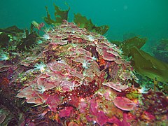  coralline algae
• 
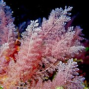  red seaweed
• 
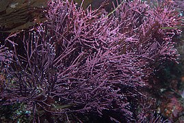  red algae
• 
  squid larva
• 
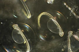  fish eggs

Evolution of the carbon cycle

Precambrian events affecting the carbon cycle 

Carbon cycle – Role of microorganisms

Microorganisms have key roles in carbon and nutrient cycling, animal (including human) and plant health, agriculture and the global food web. Microorganisms live in all environments on Earth that are occupied by macroscopic organisms, and they are the sole life forms in other environments, such as the deep subsurface and ‘extreme’ environments. Microorganisms date back to the origin of life on Earth at least 3.8 billion years ago, and they will likely exist well beyond any future extinction events... Unless we appreciate the importance of microbial processes, we fundamentally limit our understanding of Earth’s biosphere and response to climate change and thus jeopardize efforts to create an environmentally sustainable future.

A microorganism is any microscopic organism or virus not visible to the naked eye (smaller than 50 μm) that can exist in a unicellular, multicellular (for example, differentiating species), aggregate (for example, biofilm) or viral form. Examples are microscopic bacteria, archaea, eukaryotes and viruses, as well as macroscopic unicellular eukaryotes, such as larger marine phytoplankton, and wood-decomposing fungi.

Marine biome

Marine biomes cover ~70% of Earth’s surface and range from coastal estuaries, mangroves and coral reefs to the open oceans (Fig. 1). Phototrophic microorganisms use the sun’s energy in the top 200 m of the water column, whereas marine life in deeper zones uses organic and inorganic chemicals for energy10. In addition to sunlight, the availability of other energy forms and water temperature (ranging from approximately −2 °C in ice-covered seas to more than 100 °C in hydrothermal vents) influence the composition of marine communities11. Rising temperatures not only affect biological processes but also reduce water density and thereby stratification and circulation, which affect organismal dispersal and nutrient transport. Precipitation, salinity and winds also affect stratification, mixing and circulation. Nutrient inputs from air, river and estuarine flows also affect microbial community composition and function, and climate change affects all these physical factors.

The overall relevance of microorganisms to ocean ecosystems can be appreciated from their number and biomass in the water column and subsurface: the total number of cells is more than 10²⁹, and the Census of Marine Life estimates that 90% of marine biomass is microbial. Beyond their sheer numbers, marine microorganisms fulfil key ecosystem functions. By fixing carbon and nitrogen, and remineralizing organic matter, marine microorganisms form the basis of ocean food webs and thus global carbon and nutrient cycles. The sinking, deposition and burial of fixed carbon in particulate organic matter to marine sediments is a key, long-term mechanism for sequestering CO2 from the atmosphere. Therefore, the balance between regeneration of CO2 and nutrients via remineralization versus burial in the seabed determines the effect on climate change.

In addition to getting warmer (from increased atmospheric CO2 concentrations enhancing the greenhouse effect), oceans have acidified by ~0.1 pH units since preindustrial times, with further reductions of 0.3–0.4 units predicted by the end of the century. Given the unprecedented rate of pH change there is a need to rapidly learn how marine life will respond. The impact of elevated greenhouse gas concentrations on ocean temperature, acidification, stratification, mixing, thermohaline circulation, nutrient supply, irradiation and extreme weather events affects the marine microbiota in ways that have substantial environmental consequences, including major shifts in productivity, marine food webs, carbon export and burial in the seabed.

Microorganisms affect climate change

Marine phytoplankton perform half of the global photosynthetic CO₂ fixation (net global primary production of ~50 petagram C per year) and half of the oxygen production despite amounting to only ~1% of global plant biomass. In comparison with terrestrial plants, marine phytoplankton are distributed over a larger surface area, are exposed to less seasonal variation and have markedly faster turnover rates than trees (days versus decades). Therefore, phytoplankton respond rapidly on a global scale to climate variations. These characteristics are important when one is evaluating the contributions of phytoplankton to carbon fixation and forecasting how this production may change in response to perturbations. Predicting the effects of climate change on primary productivity is complicated by phytoplankton bloom cycles that are affected by both bottom-up control (for example, availability of essential nutrients and vertical mixing) and top-down control (for example, grazing and viruses). Increases in solar radiation, temperature and freshwater inputs to surface waters strengthen ocean stratification and consequently reduce transport of nutrients from deep water to surface waters, which reduces primary productivity. Conversely, rising CO₂ levels can increase phytoplankton primary production, but only when nutrients are not limiting.

Some studies indicate that overall global oceanic phytoplankton density has decreased in the past century, but these conclusions have been questioned because of the limited availability of long-term phytoplankton data, methodological differences in data generation and the large annual and decadal variability in phytoplankton production. Moreover, other studies suggest a global increase in oceanic phytoplankton production  and changes in specific regions or specific phytoplankton groups. The global sea ice (Sea Ice Index) is declining, leading to higher light penetration and potentially more primary production; however, there are conflicting predictions for the effects of variable mixing patterns and changes in nutrient supply and for productivity trends in polar zones. This highlights the need to collect long-term data on phytoplankton production and microbial community composition. Long-term data are needed to reliably predict how microbial functions and feedback mechanisms will respond to climate change, yet only very few such datasets exist (for example, the Hawaii Ocean Time-series and the Bermuda Atlantic Time-series Study). In this context, the Global Ocean Sampling Expedition, transects of the Southern Ocean, and the Tara Oceans Consortium  provide metagenome data that are a valuable baseline of marine microorganisms.

Diatoms perform 25–45% of total primary production in the oceans, owing to their prevalence in open-ocean regions when total phytoplankton biomass is maximal. Diatoms have relatively high sinking speeds compared with other phytoplankton groups, and they account for ~40% of particulate carbon export to depth. Physically driven seasonal enrichments in surface nutrients favour diatom blooms. Anthropogenic climate change will directly affect these seasonal cycles, changing the timing of blooms and diminishing their biomass, which will reduce primary production and CO2 uptake. Remote sensing data suggest a global decline of diatoms between 1998 and 2012, particularly in the North Pacific, which is associated with shallowing of the surface mixed layer and lower nutrient concentrations.

In addition to the contribution of marine phytoplankton to CO2 sequestration, chemolithoautotrophic archaea and bacteria fix CO₂ under dark conditions in deep ocean waters  and at the surface during polar winter. Marine bacteria and archaea also contribute substantially to surface ocean respiration and cycling of many elements. Seafloor methanogens and methanotrophs are important producers and consumers of CH₄, but their influence on the atmospheric flux of this greenhouse gas is uncertain. Marine viruses, bacteriovorous bacteria and eukaryotic grazers are also important components of microbial food webs; for example, marine viruses influence how effectively carbon is sequestered and deposited into the deep ocean. Climate change affects predator–prey interactions, including virus–host interactions, and thereby global biogeochemical cycles.

Oxygen minimum zones (OMZs) have expanded in the past 50 years as a result of ocean warming, which reduces oxygen solubility. OMZs are global sinks for reactive nitrogen, and microbial production of N₂ and N₂O accounts for ~25–50% of nitrogen loss from the ocean to the atmosphere. Furthermore, OMZs are the largest pelagic methane reservoirs in the ocean and contribute substantially to open ocean methane cycling. The observed and predicted future expansion of OMZs may therefore considerably affect ocean nutrient and greenhouse gas budgets, and the distributions of oxygen-dependent organisms.

The top 50 cm of deep-sea sediments contains ~1 × 10²⁹ microorganisms, and the total abundances of archaea and bacteria in these sediments increase with latitude (from 34° N to 79° N) with specific taxa (such as Marine Group I Thaumarchaeota) contributing disproportionately to the increase. Benthic microorganisms show biogeographic patterns and respond to variations in the quantity and quality of the particulate matter sinking to the seafloor. As a result, climate change is expected to particularly affect the functional processes that deep-sea benthic archaea perform (such as ammonia oxidation) and associated biogeochemical cycles.

Aerosols affect cloud formation, thereby influencing sunlight irradiation and precipitation, but the extent to which and the manner in which they influence climate remains uncertain. Marine aerosols consist of a complex mixture of sea salt, non-sea-salt sulfate and organic molecules and can function as nuclei for cloud condensation, influencing the radiation balance and, hence, climate. For example, biogenic aerosols in remote marine environments (for example, the Southern Ocean) can increase the number and size of cloud droplets, having similar effects on climate as aerosols in highly polluted regions. Specifically, phytoplankton emit dimethylsulfide, and its derivate sulfate promotes cloud condensation. Understanding the ways in which marine phytoplankton contribute to aerosols will allow better predictions of how changing ocean conditions will affect clouds and feed back on climate84. In addition, the atmosphere itself contains ~10²² microbial cells, and determining the ability of atmospheric microorganisms to grow and form aggregates will be valuable for assessing their influence on climate.

Vegetated coastal habitats are important for carbon sequestration, determined by the full trophic spectrum from predators to herbivores, to plants and their associated microbial communities. Human activity, including anthropogenic climate change, has reduced these habitats over the past 50 years by 25–50%, and the abundance of marine predators has dropped by up to 90%. Given such extensive perturbation, the effects on microbial communities need to be evaluated because microbial activity determines how much carbon is remineralized and released as CO₂ and CH₄.

Climate change affects microorganisms

Climate change perturbs interactions between species and forces species to adapt, migrate and be replaced by others or go extinct28,88. Ocean warming, acidification, eutrophication and overuse (for example, fishing, tourism) together cause the decline of coral reefs and may cause ecosystems shifts towards macroalgae89,90,91,92,93 and benthic cyanobacterial mats94,95. The capacity for corals to adapt to climate change is strongly influenced by the responses of their associated microorganisms, including microalgal symbionts and bacteria96,97,98. The hundreds to thousands of microbial species that live on corals are crucial for host health, for example by recycling the waste products, by provisioning essential nutrients and vitamins and by assisting the immune system to fight pathogens99. However, environmental perturbation or coral bleaching can change the coral microbiome rapidly. Such shifts undoubtedly influence the ecological functions and stability of the coral–microorganism system, potentially affecting the capacity and pace at which corals adapt to climate change, and the relationships between corals and other components of the reef ecosystem99,100.

Generally, microorganisms can disperse more easily than macroscopic organisms. Nevertheless, biogeographic distinctions occur for many microbial species, with dispersal, lifestyle (for example, host association) and environmental factors strongly influencing community composition and function54,101,102,103. Ocean currents and thermal and latitudinal gradients are particularly important for marine communities104,105. If movement to more favourable environments is impossible, evolutionary change may be the only survival mechanism88. Microorganisms, such as bacteria, archaea and microalgae, with large population sizes and rapid asexual generation times have high adaptive potential22. Relatively few studies have examined evolutionary adaptation to ocean acidification or other climate change-relevant environmental variables22,28. Similarly, there is limited understanding of the molecular mechanisms of physiological responses and the implications of those responses for biogeochemical cycles.18,

However, several studies have demonstrated effects of elevated CO2 levels on individual phytoplankton species, which may disrupt broader ecosystem-level processes. A field experiment demonstrated that increasing CO2 levels provide a selective advantage to a toxic microalga, Vicicitus globosus, leading to disruption of organic matter transfer across trophic levels106. The marine cyanobacterial genus Trichodesmium responds to long-term (4.5-year) exposure to elevated CO2 levels with irreversible genetic changes that increase nitrogen fixation and growth107. For the photosynthetic green alga Ostreococcus tauri, elevated CO2 levels increase growth, cell size and carbon-to-nitrogen ratios108. Higher CO2 levels also affect the population structure of O. tauri, with changes in ecotypes and niche occupation, thereby affecting the broader food webs and biogeochemical cycles108. Rather than producing larger cells, the calcifying phytoplankton species Emiliania huxleyi responds to the combined effects of elevated temperature and elevated CO2 levels (and associated acidification) by producing smaller cells that contain less carbon109. However, for this species, overall production rates do not change as a result of evolutionary adaptation to higher CO2 levels109. Responses to CO2 levels differ between communities (for example, between Arctic phytoplankton and Antarctic phytoplankton110). A mesocosm study identified variable changes in the diversity of viruses that infect E. huxleyi when it is growing under elevated CO2 levels, and noted the need to determine whether elevated CO2 levels directly affected viruses, hosts or the interactions between them111. These examples illustrate the need to improve our understanding of evolutionary processes and incorporate that knowledge into predictions of the effects of climate change.

Ocean acidification presents marine microorganisms with pH conditions well outside their recent historical range, which affects their intracellular pH homeostasis18,112. Species that are less adept at regulating internal pH will be more affected, and factors such as organism size, aggregation state, metabolic activity and growth rate influence the capacity for regulation112.

Lower pH causes bacteria and archaea to change gene expression in ways that support cell maintenance rather than growth18. In mesocosms with low phytoplankton biomass, bacteria committed more resources to pH homeostasis than bacteria in nutrient-enriched mesocosms with high phytoplankton biomass. Consequently, ocean acidification is predicted to alter the microbial food web via changes in cellular growth efficiency, carbon cycling and energy fluxes, with the biggest effects expected in the oligotrophic regions, which include most of the ocean18. Experimental comparisons of Synechococcus sp. growth under both present and predicted future pH concentrations showed effects not only on the cyanobacteria but also on the cyanophage viruses that infect them113.

Environmental temperature and latitude correlate with the diversity, distribution and/or temperature optimum (Topt) of certain marine taxa, with models predicting that rising temperatures will cause a poleward shift of cold-adapted communities52,114,115,116,117,118. However, Topt of phytoplankton from polar and temperate waters was found to be substantially higher than environmental temperatures, and an eco-evolutionary model predicted that Topt for tropical phytoplankton would be substantially higher than observed experimental values116. Understanding how well microorganisms are adapted to environmental temperature and predicting how they will respond to warming requires assessments of more than Topt, which is generally a poor indicator of physiological and ecological adaptation of microorganisms from cold environments119.

Many environmental and physiological factors influence the responses and overall competitiveness of microorganisms in their native environment. For example, elevated temperatures increase protein synthesis in eukaryotic phytoplankton while reducing cellular ribosome concentration120. As the biomass of eukaryotic phytoplankton is ~1 Gt C (ref.13) and ribosomes are phosphate rich, climate change-driven alteration of their nitrogen-to-phosphate ratio will affect resource allocation in the global ocean120. Ocean warming is thought to favour smaller plankton types over larger ones, changing biogeochemical fluxes such as particle export121. Increased ocean temperatures, acidification and decreased nutrient supplies are projected to increase the extracellular release of dissolved organic matter from phytoplankton, with changes in the microbial loop possibly causing increased microbial production at the expense of higher trophic levels122. Warming can also alleviate iron limitation of nitrogen-fixing cyanobacteria, with potentially profound implications for new nitrogen supplied to food webs of the future warming oceans123. Careful attention needs to be paid to how to quantify and interpret responses of environmental microorganisms to ecosystem changes and stresses linked to climate change124,125. Key questions thus remain about the functional consequences of community shifts, such as changes in carbon remineralization versus carbon sequestration, and nutrient cycling.

Terrestrial biome

There is ~100-fold more terrestrial biomass than marine biomass, and terrestrial plants account for a large proportion of Earth’s total biomass15. Terrestrial plants perform roughly half of net global primary production30,67. Soils store ~2,000 billion tonnes of organic carbon, which is more than the combined pool of carbon in the atmosphere and vegetation126. The total number of microorganisms in terrestrial environments is ~1029, similar to the total number in marine environments8. Soil microorganisms regulate the amount of organic carbon stored in soil and released back to the atmosphere, and indirectly influence carbon storage in plants and soils through provision of macronutrients that regulate productivity (nitrogen and phosphorus)126,127. Plants provide a substantial amount of carbon to their mycorrhizal fungal symbionts, and in many ecosystems, mycorrhizal fungi are responsible for substantial amounts of nitrogen and phosphorus acquisition by plants128.

Plants remove CO2 from the atmosphere through photosynthesis and create organic matter that fuels terrestrial ecosystems. Conversely, autotrophic respiration by plants (60 Pg C per year) and heterotrophic respiration by microorganisms (60 Pg C per year) release CO2 back into the atmosphere126,129. Temperature influences the balance between these opposing processes and thus the capacity of the terrestrial biosphere to capture and store anthropogenic carbon emissions (currently, storing approximately one quarter of emissions) (Fig. 1). Warming is expected to accelerate carbon release into the atmosphere129.

Forests cover ~30% of the land surface, contain ~45% of terrestrial carbon, make up ~50% of terrestrial primary production and sequester up to 25% of anthropogenic CO2 (refs130,131). Grasslands cover ~29% of the terrestrial surface132. Non-forested, arid and semiarid regions (47%) are important for the carbon budget and respond differently to anthropogenic climate change than forested regions132,133. Lakes make up ~4% of the non-glaciated land area134, and shallow lakes emit substantial amounts of CH4 (refs135,136). Peat (decomposed plant litter) covers ~3% of the land surface and, due to plant productivity exceeding decomposition, intact peatlands function as a global carbon sink and contain ~30% of global soil carbon137,138. In permafrost, the accumulation of carbon in organic matter (remnants of plants, animals and microorganisms) far exceeds the respiratory losses, creating the largest terrestrial carbon sink139,140,141. Climate warming of 1.5–2 °C (relative to the global mean surface temperature in 1850–1900) is predicted to reduce permafrost by 28–53% (compared with levels in 1960–1990)142, thereby making large carbon reservoirs available for microbial respiration and greenhouse gas emissions.

Evaluations of the top 10 cm of soil143 and whole-soil profiles to 100 cm deep, which contain older stocks of carbon144, demonstrate that warming increases carbon loss to the atmosphere. Explaining differences in carbon loss between different soil sites will require a greater range of predictive variables (in addition to soil organic matter content, temperature, precipitation, pH and clay content)145,146. Nevertheless, predictions from global assessments of responses to warming indicate that terrestrial carbon loss under warming is causing a positive feedback that will accelerate the rate of climate change143, particularly in cold and temperate soils, which store much of the global soil carbon147.

Microorganisms affect climate change

Higher CO2 levels in the atmosphere increase primary productivity and thus forest leaf and root litter148,149,150, which leads to higher carbon emissions due to microbial degradation151. Higher temperatures promote higher rates of terrestrial organic matter decomposition152. The effect of temperature is not just a kinetic effect on microbial reaction rates but results from plant inputs stimulating microbial growth152,153,154.

Several local environmental factors (such as microbial community composition, density of dead wood, nitrogen availability and moisture) influence rates of microbial activity (for example, fungal colonization of wood) necessitating Earth system model predictions of soil carbon losses through climate warming to incorporate local controls on ecosystem processes155. In this regard, plant nutrient availability affects the net carbon balance in forests, with nutrient-poor forests releasing more carbon than nutrient-rich forests156. Microbial respiration may be lower in nutrient-rich forests as plants provide less carbon (for example, as root exudates) to rhizosphere microorganisms157.

Plants release ~50% of fixed carbon into the soil, which is available for microbial growth158,159,160. In addition to microorganisms using exudates as an energy source, exudates can disrupt mineral–organic associations, liberating organic compounds from minerals that are used for microbial respiration, thereby increasing carbon release159. The relevance of these plant–mineral interactions illustrates the importance of biotic–abiotic interactions, in addition to biotic interactions (plant–microorganism) when one is evaluating the influence of climate change159. Thermodynamic models that incorporate the interactions of microorganisms and secreted enzymes with organic matter and minerals have been used to predict soil carbon–climate feedbacks in response to increasing temperature; one study predicted more variable but weaker soil carbon–climate feedbacks from a thermodynamic model than from static models160.

The availability of soil organic matter for microbial degradation versus long-term storage depends on many environmental factors, including the soil mineral characteristics, acidity and redox state; water availability; climate; and the types of microorganisms present in the soil161. The nature of the organic matter, in particular substrate complexity, affects microbial decomposition. Furthermore, the microbial capacity to access organic matter differs between soil types (for example, with different clay content)162. If access is taken into account, increasing atmospheric CO2 levels are predicted to allow greater microbial decomposition and less soil retention of organic carbon162.

Elevated CO2 concentrations enhance competition for nitrogen between plants and microorganisms163. Herbivores (invertebrates and mammals) affect the amount of organic matter that is returned to soil and thereby microbial biomass and activity164. For example, grasshoppers diminish plant biomass and plant nitrogen demand, thereby increasing microbial activity163. Climate change can reduce herbivory, resulting in overall alterations to global nitrogen and carbon cycles that reduce terrestrial carbon sequestration163. Detritivores (for example, earthworms) influence greenhouse gas emissions by indirectly affecting plants (for example, by increasing soil fertility) and soil microorganisms165. Earthworms modify soils through feeding, burrowing and deposition of waste products. The anaerobic gut environment of earthworms harbours microorganisms that perform denitrification and produce N2O. Earthworms enhance soil fertility, and their presence can result in net greenhouse gas emissions165, although the combined effects of increased temperature and decreased rainfall on detritivore feeding and microbial respiration may reduce emissions166.

In peatlands, decay-resistant litter (for example, antimicrobial phenolics and polysaccharides of Sphagnum mosses) inhibits microbial decomposition, and water saturation restricts oxygen exchange and promotes the growth of anaerobes and release of CO2 and CH4 (refs137,167). Increased temperature and reduced soil water content caused by climate change promote the growth of vascular plants (ericaceous shrubs) but reduce the productivity of peat moss. Changes in plant litter composition and associated microbial processes (for example, reduced immobilization of nitrogen and enhanced heterotrophic respiration) are switching peatlands from carbon sinks to carbon sources137.

Melting and degradation of permafrost allows microbial decomposition of previously frozen carbon, releasing CO2 and CH4 (refs139,140,141,168,169). Coastal permafrost erosion will lead to the mobilization of large quantities of carbon to the ocean, with potentially large CO2 emissions occurring through increased microbial remineralization170, causing a positive feedback loop that accelerates climate change139,140,141,168,169,170,171. Melting of permafrost leads to increases in water-saturated soils172, which promotes anaerobic CH4 production by methanogens and CO2 production by a range of microorganisms. Production is slow compared with metabolism in drained aerobic soils, which release CO2 rather than CH4. However, a 7-year laboratory study of CO2 and CH4 production found that once methanogen communities became active in thawing permafrost, equal amounts of CO2 and CH4 were formed under anoxic conditions, and it was predicted that by the end of the century, carbon emissions from anoxic environments will drive climate change to a greater extent than emissions from oxic environments172.

A 15-year mesocosm study that simulated freshwater lake environments determined that the combined effects of eutrophication and warming can lead to large increases in CH4 ebullition (bubbles from accumulated gas)135. As small lakes are susceptible to eutrophication and tend to be located in climate-sensitive regions, the role of lake microorganisms in contributing to global greenhouse gas emissions needs to be evaluated135,136.

Climate change affects microorganisms

Shifts in climate can influence the structure and diversity of microbial communities directly (for example, seasonality and temperature) or indirectly (for example, plant composition, plant litter and root exudates). Soil microbial diversity influences plant diversity and is important for ecosystem functions, including carbon cycling173,174.

Both short-term laboratory warming and long-term (more than 50 years) natural geothermal warming initially increased the growth and respiration of soil microorganisms, leading to net CO2 release and subsequent depletion of substrates, causing a decrease in biomass and reduced microbial activity175. This implies that microbial communities do not readily adapt to higher temperatures, and the resulting effects on reaction rates and substrate depletion reduce overall carbon loss175. By contrast, a 10-year study found that soil communities adapted to increased temperature by changing composition and patterns of substrate use, leading to less carbon loss than would have occurred without adaptation176. Substantial changes in bacterial and fungal communities were also found in forest soils with a more than 20 °C average annual temperature range177, and in response to warming across a 9-year study of tall-grass prairie soils178.

Two studies assessed the effects of elevated temperatures on microbial respiration rates and mechanisms and outcomes of adaptation179,180. The studies examined a wide range of environmental temperatures (−2 to 28 °C), dryland soils (110 samples) and boreal, temperate and tropical soils (22 samples), and evaluated how communities respond to three different temperatures (~10–30 °C). Thermal adaptation was linked to biophysical characteristics of cell membranes and enzymes (reflecting activity-stability trade-offs180) and the genomic potential of microorganisms (with warmer environments having microbial communities with more diverse lifestyles179). Respiration rates per unit biomass were lower in soils from higher-temperature environments, indicating that thermal adaptation of microbial communities may lessen positive climate feedbacks. However, as respiration depends on multiple interrelated factors (not just on one variable, such as temperature), such mechanistic insights into microbial physiology need to be represented in biogeochemical models of possible positive climate feedbacks.

Microbial growth responses to temperature change are complex and varied181. Microbial growth efficiency is a measure of how effectively microorganisms convert organic matter into biomass, with lower efficiency meaning more carbon is released to the atmosphere182,183. A 1-week laboratory study found that increasing temperature led to increases in microbial turnover but no change in microbial growth efficiency, and predicted that warming would promote carbon accumulation in soil183. A field study spanning 18 years found microbial efficiency was reduced at higher soil temperature, with decomposition of recalcitrant, complex substrates increasing by the end of the period along with a net loss of soil carbon182.

Similarly, in a 26-year forest-soil warming study, temporal variation occurred in organic matter decomposition and CO2 release184, leading to changes in microbial community composition and carbon use efficiency, reduced microbial biomass and reduced microbially accessible carbon184. Overall, the study predicted anthropogenic climate change to cause long-term, increasing and sustained carbon release184. Similar predictions arise from Earth system models that simulate microbial physiological responses185 or incorporate the effects of freezing and thawing of cold-climate soils186.

Climate change directly and indirectly influences microbial communities and their functions through several interrelated factors, such as temperature, precipitation, soil properties and plant input. As soil microorganisms in deserts are carbon limited, increased carbon input from plants promotes transformation of nitrogenous compounds, microbial biomass, diversity (for example, of fungi), enzymatic activity and use of recalcitrant organic matter133. Although these changes may enhance respiration and net loss of carbon from soil, the specific characteristics of arid and semiarid regions may mean they could function as carbon sinks133. However, a study of 19 temperate grassland sites found that seasonal differences in rainfall constrain biomass accumulation132. To better understand aboveground plant-biomass responses to CO2 levels and seasonal precipitation, we also need improved knowledge of microbial community responses and functions.

Metagenome data, including metagenome-assembled genomes, provide knowledge of key microbial groups that metabolize organic matter and release CO2 and CH4 and link these groups to the biogeochemistry occurring in thawing permafrost187,188,189,190,191. Tundra microbial communities change in the soil layer of permafrost after warming192. Within 1.5 years of warming, the functional potential of the microbial communities changed markedly, with an increasing abundance of genes involved in aerobic and anaerobic carbon decomposition and nutrient cycling. Although microbial metabolism stimulates primary productivity by plants, the balance between microbial respiration and primary productivity results in a net release of carbon to the atmosphere192. When forests expand into warming regions of tundra, plant growth can produce a net loss of carbon, possibly as a result of root exudates stimulating microbial decomposition of native soil carbon153,193. Although there are reports of carbon accumulating owing to warming (for example, ref.183), most studies describe microbial community responses that result in carbon loss.

Rapid warming of the Antarctic Peninsula and associated islands resulted in range expansion of Antarctic hair grass (Deschampsia antarctica), as it outcompetes other indigenous species (for example, the moss Sanionia uncinata) through the superior capacity of its roots to acquire peptides and thus nitrogen194. The ability of the grass to be competitive depends on microbial digestion of extracellular proteins and generation of amino acids, nitrate and ammonium194. As warmer soils in this region harbour greater fungal diversity, climate change is predicted to cause changes in the fungal communities that will affect nutrient cycling and primary productivity195. Cyanobacterial diversity and toxin production within benthic mats from both the Antarctic Peninsula and the Arctic increased during 6 months of exposure to high growth temperatures196. A shift to toxin-producing species or increased toxin production by existing species could affect polar freshwater lakes, where cyanobacteria are often the dominant benthic primary producers196.

Conclusion

Microorganisms make a major contribution to carbon sequestration, particularly marine phytoplankton, which fix as much net CO2 as terrestrial plants. For this reason, environmental changes that affect marine microbial photosynthesis and subsequent storage of fixed carbon in deep waters are of major importance for the global carbon cycle. Microorganisms also contribute substantially to greenhouse gas emissions via heterotrophic respiration (CO2), methanogenesis (CH4) and denitrification (N2O).

Many factors influence the balance of microbial greenhouse gas capture versus emission, including the biome, the local environment, food web interactions and responses, and particularly anthropogenic climate change and other human activities (Figs 1–3).

Human activity that directly affects microorganisms includes greenhouse gas emissions (particularly CO2, CH4 and N2O), pollution (particularly eutrophication), agriculture (particularly land usage) and population growth, which positively feeds back on climate change, pollution, agricultural practice and the spread of disease. Human activity that alters the ratio of carbon uptake relative to release will drive positive feedbacks and accelerate the rate of climate change. By contrast, microorganisms also offer important opportunities for remedying human-caused problems through improved agricultural outcomes, production of biofuels and remediation of pollution.

Protist shell

"The amoebae also are extremely diverse. Amoebae are defined based on pseudopodia type: those with thin, or filose, pseudopods, which may be reinforced by stiff microtubule proteins, are classified in the supergroup Rhizaria (e.g., foraminiferans and radiolarians), whereas those with lobose pseudopods, which are blunt and are not reinforced, are classified in the supergroup Amoebozoa. Both groups of amoebae can be “naked” or housed inside a shell, or test, composed of organic or inorganic materials.The naked amoebae are the simplest of the amoebae. They have no defined shape and extend one or many lobose pseudopodia. Many of these lobose amoebae, including those in the genera Mastigamoeba and Mastigella, also possess flagella in the vegetative (resting) phase. At the opposite extreme are the complex foraminiferans, which live inside multichambered calcareous shells up to several millimetres in diameter. The filose pseudopodia of foraminiferans are known as reticulopodia and extend from the aperture of the largest chamber of the shell, forming a complicated, sticky branching network. Rhizarian amoebae that are known commonly as radiolarians form shells from silica or strontium sulfate; in some the shell has so many holes that the structure resembles a sponge. The polyphyletic heliozoans, or sun protozoans, have radiating pseudopodia (axopodia) that extend like spokes from the central body; microtubules support an outer layer of cytoplasm. Many heliozoans are members of Rhizaria; however, some are placed in Chromalveolata."

Dinoflagellates

See also: Mixotrophic dinoflagellate and Predatory dinoflagellate

Dinoflagellate shapes

Unarmored dinoflagellates Kofoid (1921)

Haeckel Peridinea (1904)

Dinoflagellates are part of the algae group, and form a phylum of unicellular flagellates with about 2,000 marine species. The name comes from the Greek "dinos" meaning whirling and the Latin "flagellum" meaning a whip or lash. This refers to the two whip-like attachments (flagella) used for forward movement. Most dinoflagellates are protected with red-brown, cellulose armour. Like other phytoplankton, dinoflagellates are r-strategists which under right conditions can bloom and create red tides. Excavates may be the most basal flagellate lineage.

By trophic orientation dinoflagellates cannot be uniformly categorized. Some dinoflagellates are known to be photosynthetic, but a large fraction of these are in fact mixotrophic, combining photosynthesis with ingestion of prey (phagotrophy). Some species are endosymbionts of marine animals and other protists, and play an important part in the biology of coral reefs. Others predate other protozoa, and a few forms are parasitic. Many dinoflagellates are mixotrophic and could also be classified as phytoplankton.

• 
  Gyrodinium, one of the few naked dinoflagellates which lack armour
• 
  The dinoflagellate Dinophysis acuta

Dinoflagellates

        Armoured

        Unarmoured

Traditionally dinoflagellates have been presented as armoured or unarmoured

• 
  Tripos muelleri is recognisable by its U-shaped horns

Amoeba

Shelled and naked amoeba

Testate amoeba, Cyphoderia sp.

Naked amoeba, Chaos sp.

                  Amoeba can be shelled (testate) or naked

• 
  Naked amoeba showing food vacuoles and ingested diatom
• 
  Shell or test of a testate amoeba, Arcella sp.
• 
  Xenogenic testate amoeba covered in diatoms (from Penard's Amoeba Collection)

Amoeba engulfing a diatom

Ciliates

• 
  Tintinnopsis campanula
• 
  Oxytricha chlorelligera
• 
  Stylonychia putrina
• 
  Holophyra ovum
• 
  Blepharisma japonicum

Ciliate shapes

          Drawings by Haeckel 1904 (click for details)

• 
  Mesodinium rubrum produce deep red blooms using enslaved chloroplasts from their algal prey 
• Several taxa of ciliates interacting
• Blepharisma americanum swimming in a drop of pond water with other microorganisms

• Mixoplankton
• 
  Tintinnid ciliate Favella
• 
  Euglena mutabilis, a photosynthetic flagellate
• 
  Zoochlorellae (green) living inside the ciliate Stichotricha secunda

Other taxa

Triparma laevis and a drawing of its silicate shell, scale bar = 1 μm.

Exploded drawing of the shell, D = dorsal plate, G = girdle plate, S = shield plate and V = ventral plate.

Triparma laevis belongs to the Bolidophyceae, a sister taxon to the diatoms.

Microfossils

An overview of sediment core collection and processing for micropaleontological research

(b) Ocean-floor sediment samples collected with a dredge during the HMS Challenger expedition on March 21, 1876, in the South Atlantic. Sample number M.408 from the Ocean-Bottom Deposit (OBD) Collection held by the Natural History Museum in London. (c) Sand-sized residue of a Pleistocene deep-sea sediment from ODP Site 925 in the equatorial Atlantic Ocean consisting of numerous microfossil shells.            Scale bar: 1 mm

See also: Marine biogeochemical cycles

Further information: Calcareous ooze, Biogenic silica, Radiolarite, Sedimentary rock, Microfossil, and Reverse weathering

Sediments at the bottom of the ocean have two main origins, terrigenous and biogenous.

Terrigenous sediments account for about 45% of the total marine sediment, and originate in the erosion of rocks on land, transported by rivers and land runoff, windborne dust, volcanoes, or grinding by glaciers.

Biogenous sediments account for the other 55% of the total sediment, and originate in the skeletal remains of marine protists (single-celled plankton and benthos microorganisms). Much smaller amounts of precipitated minerals and meteoric dust can also be present. Ooze, in the context of a marine sediment, does not refer to the consistency of the sediment but to its biological origin. The term ooze was originally used by John Murray, the "father of modern oceanography", who proposed the term radiolarian ooze for the silica deposits of radiolarian shells brought to the surface during the Challenger Expedition. A biogenic ooze is a pelagic sediment containing at least 30 percent from the skeletal remains of marine organisms.

Thickness of marine sediments

Main types of biogenic ooze
type	mineral forms	protist involved		name of skeleton	typical size (mm)
Siliceous ooze	SiO2 silica quartz glass opal chert	diatom		frustule	0.002 to 0.2		diatom microfossil from 40 million years ago
		radiolarian		test or shell	0.1 to 0.2		elaborate silica shell of a radiolarian
Calcareous ooze	CaCO3 calcite aragonite limestone marble chalk	foraminiferan		test or shell	under 1		Calcified test of a planktic foraminiferan. There are about 10,000 living species of foraminiferans
		coccolithophore		coccoliths	under 0.1		Coccolithophores are the largest global source of biogenic calcium carbonate, and significantly contribute to the global carbon cycle. They are the main constituent of chalk deposits such as the white cliffs of Dover.

• 
  Diatomaceous earth is a soft, siliceous, sedimentary rock made up of microfossils in the form of the frustules (shells) of single cell diatoms (click to magnify)
• 
  Illustration of a Globigerina ooze
• 
  Shells (tests), usually made of calcium carbonate, from a foraminiferal ooze on the deep ocean floor

Stone dagger of Ötzi the Iceman who lived during the Copper Age. The blade is made of chert containing radiolarians, calcispheres, calpionellids and a few sponge spicules. The presence of calpionellids, which are extinct, was used to date this dagger.

• 
  Opal can contain protist microfossils of diatoms, radiolarians, silicoflagellates and ebridians
• 
  Marble can contain protist microfossils of foraminiferans, coccolithophores, calcareous nannoplankton and algae, ostracodes, pteropods, calpionellids and bryozoa
• 
  Carbonate-silicate cycle

Calcareous microfossils from marine sediment consisting mainly of star-shaped discoaster with a sprinkling of coccoliths

Distribution of sediment types on the seafloor
Within each colored area, the type of material shown is what dominates, although other materials are also likely to be present.
For further information, see here

Further references

• Xu, K., Hutchins, D. and Gao, K. (2018) "Coccolith arrangement follows Eulerian mathematics in the coccolithophore Emiliania huxleyi". PeerJ, 6: e4608. doi:10.1126/science.aaa7378.

Marine coastal ecosystems

Global distribution of coral, mangrove, and seagrass diversity

Ecosystem services delivered by epibenthic bivalve reefs

Reefs provide coastal protection through erosion control and shoreline stabilization, and modify the physical landscape by ecosystem engineering, thereby providing habitat for species by facilitative interactions with other habitats such as tidal flat benthic communities, seagrasses and marshes.

references

Valuation of marine ecosystems

Interacting components for evaluating marine ecosystem services and biodiversity 

references

Bacteria morphology

Different shapes of bacteria and their sizes compared with the width of a human hair. The unit “μm” is a measurement of length, the “micrometer”, and equals 1/10,000 of a centimeter.

Bacteria display a large diversity of cellular morphologies and arrangements.

Main article: Bacterial cellular morphologies

FROM: Coccus...
A coccus (plural cocci) is any bacterium or archaeon that has a spherical, ovoid, or generally round shape. Bacteria are categorized based on their shapes into three classes: cocci (spherical-shaped), bacillus (rod-shaped) and spirochetes (spiral-shaped) cells. Coccus refers to the shape of the bacteria, and can contain multiple genera, such as staphylococci or streptococci. Cocci can grow in pairs, chains, or clusters, depending on their orientation and attachment during cell division. Contrast to many bacilli-shaped bacteria, most cocci bacteria do not have flagella and are non-motile.

FROM Bacillus (shape)...
A bacillus (plural bacilli), or bacilliform bacterium, is a rod-shaped bacterium or archaeon. Bacilli are found in many different taxonomic groups of bacteria. However, the name Bacillus, capitalized and italicized, refers to a specific genus of bacteria. The name Bacilli, capitalized but not italicized, can also refer to a less specific taxonomic group of bacteria that includes two orders, one of which contains the genus Bacillus. When the word is formatted with lowercase and not italicized, 'bacillus', it will most likely be referring to shape and not to the genus at all. Bacilliform bacteria are also often simply called rods when the bacteriologic context is clear.

FROM Spiral bacteria...
Spiral bacteria, bacteria of spiral (helical) shape, form the third major morphological category of prokaryotes along with the rod-shaped bacilli and round cocci. Spiral bacteria can be subclassified by the number of twists per cell, cell thickness, cell flexibility, and motility. The two types of spiral cells are spirillum and spirochete, with spirillum being rigid with external flagella, and spirochetes being flexible with internal flagella.

references

Freshwater fungi

NEEDS PARAPHRASING...
"Molecular diversity of microbial eukaryotes in aquatic ecosystems is far less investigated than their prokaryotic counterparts. This is even more striking for particular groups such as fungi that attract very little interest. This bias partly results from their supposed low abundances (e.g., ∼1% of total marine eukaryotes (Massana & Pedros-Alio, 2008)) that suggests fungi have little ecological importance in aquatic ecosystems. However, rare organisms can play crucial roles in ecosystem functioning but more importantly recent studies have revealed much larger proportions of fungi than previously observed, as well as high taxonomic richness in different marine (Le Calvez et al., 2009; Gao, Johnson & Wang, 2010; Orsi, Biddle & Edgcomb, 2013; Richards et al., 2012; Lepère et al., 2015) and freshwaters environments (Monchy et al., 2011; Ishii, Ishida & Kagami, 2015; Duarte et al., 2015; Lepère et al., 2016). The extent of fungal biodiversity is therefore likely underestimated (Scheffers et al., 2012) though diversity estimates based on molecular data suggest that it can range between 0.5 and 10 million species (Hawksworth, 2001; O’Brien et al., 2005; Mora et al., 2011; Bass & Richards, 2011; Blackwell, 2011)."

NEEDS PARAPHRASING...
"Despite this putative rich biodiversity, functional roles of aquatic fungi, for which only 3,000–4,000 species have been recorded, remain poorly characterized (Pautasso, 2013; Rambold, Stadler & Begerow, 2013). They are mainly known as decomposers of leaves in rivers, mangroves and wetlands (Seena, Wynberg & Bärlocher, 2008; Gulis, Kuehn & Suberkropp, 2009) and as parasites of phytoplankton and zooplankton in lake ecosystems (Jobard, Rasconi & Sime-Ngando, 2010). A decade ago, fungi were divided into four main phyla: Basidiomycota, Ascomycota, Zygomycota and Chytridiomycota (James et al., 2006). However, phylogeny of fungi is still unresolved and several phyla, classes and orders of basal fungi have been determined, since. For example, Corradi (2015) highlighted that Cryptomycota forms a new phylum in which we can find Microsporidia, Aphelids and Rozellids. The vast majority of this phylum is characterized by environmental sequences and gathered under the term “dark matter fungi” (Grossart et al., 2015). These fungi are mostly zoosporic and “old” in term of evolution since they diverged from the remaining fungi 710–1,060 million years ago (Lücking et al., 2009). These basal fungi are distant from cultured and described fungi. Aquatic environments are thus likely to host a high number of uncharacterized groups (Grossart & Rojas-Jimenez, 2016)."

Bacterial and fungal communities (in glacier-fed streams)

Glaciers currently cover about 10% of land area, and most are expected to be gone by 2050

Glacier-fed stream

NEEDS PARAPHRASING...
"Bacterial and fungal communities in biofilms are important components in driving biogeochemical processes in stream ecosystems. Previous studies have well documented the patterns of bacterial alpha diversity in stream biofilms in glacier-fed streams, where, however, beta diversity of the microbial communities has received much less attention especially considering both bacterial and fungal communities. A focus on beta diversity can provide insights into the mechanisms driving community changes associated to large environmental fluctuations and disturbances, such as in glacier-fed streams. Moreover, modularity of co-occurrence networks can reveal more ecological and evolutionary properties of microbial communities beyond taxonomic groups."

NEEDS PARAPHRASING...
"Glaciers cover approximately 10% of the land surface on the Earth (Milner et al., 2017) and are important components of the hydrological cycle providing vital water resources (Barnett, Adam & Lettenmaier, 2005; Gardner et al., 2013; Zemp et al., 2015). However, glaciers are shrinking rapidly across the world due to accelerating global warming (Immerzeel, Van Beek & Bierkens, 2010; Sorg et al., 2012; Marzeion et al., 2014), and most of them are expected to disappear by 2050 (Zemp et al., 2006; IPCC, 2014). As a prominent component of the glacier forefront, glacier-fed streams have a highly heterogeneous environment due to longitudinal alterations of landcover, river hydrology and morphology, sediment transport, and biogeochemical processes (Hood & Scott, 2008; Laghari, 2013; Hotaling, Hood & Hamilton, 2017; Milner et al., 2017). For example, from glacier terminus to downstream, terrestrial vegetation increases (Zhang et al., 2013; Raynolds et al., 2015), stream channel lengthens (Milner, Brown & Hannah, 2009; Robinson, Thompson & Freestone, 2014), and water source compositions changes (Brown, Hannah & Milner, 2003)."

The bottom of this stream is covered with bacterial biofilm (biomineralization)

Biofilm

"Stated simply, biofilms are microorganisms attached to a solid surface. Biofilms pervade virtually all environments, often dominating the microbial activity distributed between the individual planktonic and aggregated habitats"

NEEDS PARAPHRASING...
"Biofilms are hot spots of microbial diversity and activity in stream ecosystems (Geesey et al., 1978; Battin et al., 2016). Within stream biofilms, bacteria, fungi, and algae are the major components driving the bulk of metabolism and biogeochemical processes (Brittain & Milner, 2001; Battin et al., 2003; Von Schiller et al., 2007). The changing environment presents significant challenges for glacier-fed stream ecosystems. Previous studies have revealed that factors associated with glacier shrinkage have significant influences on the composition, diversity, and functional potential of bacterial communities in stream biofilms (Wilhelm et al., 2013, 2014; Ren, Gao & Elser, 2017; Ren et al., 2017). However, fungal communities in glacial systems are rarely studied (Edwards, 2015; Anesio et al., 2017). With the decrease in elevation, glacier coverage, and glacier source contribution to streamflow, as well as increase in distance to glacier terminus, bacterial communities showed increased alpha diversity as well as distinct taxonomic and functional compositions (Wilhelm et al., 2013, 2014; Ren, Gao & Elser, 2017; Ren et al., 2017)."

FROM: Biofilm...
Biofilms can be found on rocks and pebbles at the bottoms of most streams or rivers and often form on the surfaces of stagnant pools of water. Biofilms are important components of food chains in rivers and streams and are grazed by the aquatic invertebrates upon which many fish feed.

More biofilm

NEEDS PARAPHRASING...
"Streams and rivers form dense networks, shape the Earth’s surface and, in their sediments, provide an immensely large surface area for microbial growth. Biofilms dominate microbial life in streams and rivers, drive crucial ecosystem processes and contribute substantially to global biogeochemical fluxes. In turn, water flow and related deliveries of nutrients and organic matter to biofilms constitute major constraints on microbial life."

NEEDS PARAPHRASING...
"The perception that most microorganisms live as complex communities that are attached to surfaces has profoundly changed microbiology over the past decades. Most, if not all, bacteria can form biofilms, which are communities of cells embedded in a porous extracellular matrix. Dental plaque, the microorganisms on catheters and implants that cause persistent infections and the fouling of ship hulls and pipework are all examples of biofilms with important implications for public health and industrial processes. Most contemporary biofilm research rests on the discovery made more than 35 years ago by Maurice Lock, Gill Geesey and Bill Costerton: bacteria attached to surfaces dominate microbial life in streams1–3. These microbiologists pioneered research into stream biofilms, also termed periphyton or epilithon, and described them as complex aggregates of bacteria, algae, protozoa, fungi and meiobenthos. The early study of stream biofilms also highlighted the relevance of interactions between microbial phototrophs and heterotrophs for energy fluxes and the role of the biofilm matrix as the site of extracellular enzyme activity and adsorption of dissolved organic matter (DOM)3,4."

NEEDS PARAPHRASING...
"Since these early days, the study of the ecology and biogeochemistry of stream biofilms has slowly developed in the wake of thriving research on bacterial biofilms — often comprising only a single strain, of interest to medical microbiology, rather than the polymicrobial communities found in stream biofilms — and on the microbial ecology of marine and lake planktonic communities5. Unlike bacterial biofilms grown in the laboratory, biofilms in streams are continuously exposed to a diverse inoculum that includes bacteria, archaea, algae, fungi, protozoa and even metazoa. These diverse biological ‘building blocks’, when combined with the dynamic flow of streamwater, generate biofilms with inherently complex and varying physical structures that have implications for microbial functioning and ecosystem processes6. In streams, biofilms are key sites of enzymatic activity7, including organic matter cycling, ecosystem respiration and primary production and, as such, form the basis of the food web."

NEEDS PARAPHRASING...
"Why should we study the ecology and biogeochemistry of stream biofilms? Streams sculpt the continental surface, forming dense and conspicuous channel networks that can be thought of as ecological arteries that perfuse the landscape. Streams are connected to their catchments through various surface and subsurface flow paths and notably through the hyporheic zone in the streambed at the interface between groundwater and streamwater8. Microbial cells, solutes and particles enter streams through these flow paths and, en route to downstream ecosystems and ultimately to the oceans, they may interact with the biofilms that colonize the large surface area provided by the streambed as a ‘microbial skin’ (BOX 1). As a result, the streambed and its biofilm microbiome contribute to biogeochemical fluxes8. Indeed, stream biofilms are now recognized as substantial contributors to global carbon fluxes by degrading organic matter and ultimately emitting an unexpectedly large amount of carbon dioxide into the atmosphere9,10. Microorganisms in streams are also major components of the nitrogen cycle as they denitrify nitrate that they receive from catchment and emit the resulting nitrous oxide or nitrogen gas into the atmosphere11,12. Furthermore, stream biofilms can be viewed as a crucial component of the catchment microbiome that also includes the microbial communities of the phyllosphere13 and soil14. The phyllosphere and the soil crust intercept water, microorganisms and solutes upon their entry into the catchment, whereas stream biofilms regulate the export of microorganisms and solutes from the catchment. Stream biofilms thus connect the land surface, groundwater, oceans and the atmosphere, and as such they are prominently positioned at the nexus of global biogeochemistry, biodiversity and climate change."

Beta diversity

NEEDS PARAPHRASING...
"Biodiversity is important for generating and stabilizing ecosystem structure and functions (Loreau et al., 2001; Tilman, Isbell & Cowles, 2014). The positive effects of local species richness (alpha diversity) on ecosystem functioning have been widely confirmed by a growing number of studies (Chapin et al., 2000; Cardinale et al., 2012; Duffy, Godwin & Cardinale, 2017). However, comparing to alpha diversity, beta diversity is an underexplored facet of biodiversity (Mori, Isbell & Seidl, 2018), which accumulates from compositional variations among local assemblages and provides insights into the mechanisms underlining biodiversity changes and their ecological consequences (Anderson et al., 2011; Socolar et al., 2016). For ecological communities suffering intensive environmental fluctuations and disturbances, focusing on beta diversity is especially important (Mori, Isbell & Seidl, 2018). In addition, microorganisms in many environments often coexist in a complex network with positive and negative interactions among members, playing pivotal roles in community assembly (Fuhrman, 2009; Barberán et al., 2012; Shi et al., 2016). These interactions may imply biologically or biochemically meaningful relationships between microorganisms (Weiss et al., 2016). Microbial co-occurrence networks can reveal how taxa potentially interact with each other, how diverse taxa structure networks, and how networks are compartmentalized into modules of closely associated taxa, as well as how microbial communities responded to environmental variations (Newman, 2006; Fuhrman, 2009; De Menezes et al., 2015; Banerjee et al., 2016). In addition, modularity (the tendency of a network to contain sub-clusters of nodes) is an important ecological feature in many biological systems, providing opportunities to identify highly connected taxa and integrate high dimension data into predicted ecological modules (De Menezes et al., 2015; Shi et al., 2016). A module is defined as a group of densely connected operational taxonomic units (OTUs), which have less links with OTUs belonging to other modules (Shi et al., 2016), forming a clustered network topology (Barberán et al., 2012). Modules can help to reveal more ecological and evolutionary properties (Thompson, 2005; Olesen et al., 2007), which are easily overlooked when communities are studied as a whole or in taxonomic groups (Porter, Onnela & Mucha, 2009; Bissett et al., 2013; De Menezes et al., 2015). The relationships between microbial modules and environmental variables can improve our understanding of the influences of environmental variation on microbial community assembly (Lindström & Langenheder, 2012; De Menezes et al., 2015; Toju et al., 2016). However, previous studies in glacier-fed streams have only focused on the whole communities or certain taxonomic groups of bacteria and fungi (Robinson & Jolidon, 2005; Milner, Brown & Hannah, 2009; Wilhelm et al., 2013; Ren, Gao & Elser, 2017). The network and modularity features of bacterial and fungal communities in glacier-fed streams are remaining one of our knowledge gaps. Integrating beta diversity and network modularity can provide novel insights into assembly mechanisms of microbial communities in glacier-fed streams."

Biodiversity across spatial scales

NEEDS PARAPHRASING...
"Stream biofilms are jungles of biodiversity, and the organisms that are typically found within them span across the entire tree of life. The development of next-generation sequencing methods has enabled a high-throughput profiling of these biofilms that has impressively demonstrated the full breadth and complexity of their microbial diversity (FIG. 1). Depending on light availability, eukaryotic algae (such as diatoms, green algae, chrysophytes, red algae and cryptophytes) and cyanobacteria, together with bacteria and to some extent also archaea, can form biofilms in the benthic zone, whereas bacteria and archaea dominate in the deeper sediments in which phototrophic life is limited. Fungi are probably also an important component of stream biofilms but remain poorly studied15,16. Ciliates, flagellates, nematodes and even young-instar insects (such as midges) are among the top consumers in stream biofilms17,18, and their grazing activity can change the physical structure19,20, community composition21 and carbon cycling of biofilms22. Furthermore, viruses have an important role in marine ecosystems23; for example, in bacterial biofilms24, bacterial viruses (or phages) can infect cells and regulate the dynamics and diversity of bacterial communities. However, little is known of the abundance and relevance of viruses in stream biofilms."

Marine biofilm

Freshwater prokaryotes

About one third of the terrestrial organic matter (OM) that enters freshwater is sequestered in sediments.

Lake sediments

Lake sediments harbor diverse microbial communities that cycle carbon and nutrients while being constantly colonized and potentially buried by organic matter sinking from the water column.

The continuous deposition of organic and inorganic particles to sediments is an important process in all aquatic ecosystems. Approximately one third of the terrestrial organic matter (OM) that enters freshwater is sequestered in sediments, although the total amount of OM that reaches the sediments is much greater than the amount that is actually sequestered. This is because microbial activity is responsible for the cycling of carbon, including methane emission. In lake sediments, a proportion of newly settled OM is rapidly recycled and subsequently transformed into secondary compounds, resulting in a distinct uppermost sediment zone of high heterotrophic activity. This is thought to lead to the structuring of microbial communities along environmental gradients that are much steeper than those in marine sediments, with narrower vertical sequences of electron acceptors. The nature of this gradient influences the carbon, nitrogen, and sulfur cycles  and potentially affects the microbial community structure.

In contrast to the wealth of studies on marine sediments (cf. the 65 studies of, few studies have examined the vertical microbial community structure of freshwater sediments (e.g.,). The community of sediment microbes was thought to be dominated by Bacteria, together with a smaller fraction of methanogenic Archaea. This view has been challenged by the recent discovery of an abundance of non-methanogenic Archaea in marine sediments. They are assumed to be adapted to low-energy environments, and at least one lineage seems to be specialized in inter alia amino acid turnover. This discovery has led to a revised perception of microbial communities in marine sediments, where Archaea appear to be as abundant as Bacteria and increase in relative abundance with sediment depth. Data on sediment Archaea in freshwater are scarce, and the causes of the significant variation observed among studies remain largely unknown.

Prokaryotic activity, biomass, and cell numbers decrease with depth in many freshwater and marine sediments, although other studies report relatively constant proportions of active cells with depth and find no accumulation of dead cells in deeper sediments. Despite the continuous presence of vegetative cells and resting stages, recent studies of marine systems indicate that the majority of microbial cells in energy-deprived horizons consist of microbial necromass  and the proportion of living organisms decreases with the increasing age of the sediment [29]. The vertical, progressive transformation of OM and depletion of electron acceptors may eventually lead to an extremely low-energy environment in deeper sediment layers with very low growth rates similar to sub-seafloor sediments.

NEEDS PARAPHRASING...
"Lakes and ponds are the final resting place for many of the Earth’s plants. Rivers collect much of the planet’s dead organic matter, transporting it to rest in calmer waters. But on a microscopic scale, lakes are anything but calm. An invisible metropolis of microbes feeds on these logs and leaves, producing greenhouse gases as a byproduct. As a result, lakes may be responsible for as much as a quarter of the carbon in the atmosphere – and rising. New research conducted with my colleagues in Cambridge, Germany and Canada suggests that emissions from freshwater lakes could double in the coming decades because of climate change. All known life on Earth is made of carbon. When plants and animals reach the end of their lives, microorganisms such as bacteria and fungi come to feast. They feed on the carbon-based remains of other organisms and their waste products — collectively known as organic matter."

Comparison with marine prokaryotes

"Phylogenetic relationships of organisms within and across ecosystems can provide insight into the evolutionary history of lineages and how evolution might proceed into the future. Microorganisms in the water columns of freshwater and marine ecosystems provide a unique juxtaposition. On one hand, these habitats share common features of pelagic lifestyles like free-living and particle-associated niches, potential for interactions with phytoplankton, and opportunities for diverse photoheterotrophic organisms, including aerobic anoxygenic phototrophs  and rhodopsin-containing bacteria. However, salinity preference is considered a complex trait involving many genes and complex cellular integration, suggesting that transitions between high and low salinity are difficult from a genetic perspective. Consistent with this idea, microbial communities from saline environments are compositionally distinct from those inhabiting nonsaline environments. Salinity-induced shifts in microbial beta diversity have been observed in studies of marine-to-freshwater gradients in many systems, including the Baltic Sea, Columbia River Estuary system, and Antarctic lakes that have become progressively less saline since becoming isolated from the sea. These observations of ecosystem-specific diversity support the current paradigm that transitions between marine and freshwater ecosystems are infrequent, despite many ecological similarities.

Freshwater versus marine bacterial abundance by taxonomy

Median relative abundance of phyla/proteobacterial classes in freshwater and marine samples collected from surface (a) and deep (b) waters. The deepest hypolimnion (below thermocline) sample collected from stratified lakes and marine samples collected at depths >75m were classified as "deep" samples. Diagonal lines indicate a 1:1 relationship.
The abundances of phyla (classes for Proteobacteria), orders, and families between marine and freshwater samples were compared. At the phylum level, Alphaproteobacteria, Gammaproteobacteria, Euryarchaeota, and Marinimicrobia had significantly higher relative abundances in marine systems while Betaproteobacteria and Verrucomicrobia had higher relative abundances in freshwater systems.

Pairs of marine and freshwater samples sharing common taxa

Maximum sequence identity threshold (i.e., finest-scale resolution) at which pairs of marine and freshwater samples share common taxa. Box plots indicate the median, quartiles, and range of values observed for all marine-freshwater sample pairs. Colored boxes indicate phyla/proteobacterial classes that contain 5 or more shared MED nodes while gray boxes indicate groups that contain 1 to 3 shared MED nodes. The heatmap to the right illustrates the number of freshwater (F) and marine (M) samples containing representatives of each phylum/proteobacterial class. *, Actinobacteria cutoff values were calculated with a preclustered data set.

"Environmental sequence data provide support for a "salty divide" separating marine and freshwater microbial assemblages. From a phylogenetic perspective, each clade that contains both marine and freshwater representatives includes at least one transition where a common ancestor gave rise to a daughter lineage able to survive and proliferate in a new salinity environment. Transitions that occurred recently are expected to result in highly similar molecular sequences recovered from marine and freshwater systems while transitions that occurred in the distant past are expected to yield habitat-specific diversification — clades that are only observed in one habitat type or the other — and a greater sequence divergence between marine and freshwater representatives. Prior work using phylogenetic patterns concluded that transitions between marine and freshwater environments are infrequent and most transition events occurred a long time ago in evolutionary terms. For example, Logares and colleagues  found that within the abundant alphaproteobacterial SAR11 group, freshwater representatives belonged exclusively to a single subclade, called LD12, implying a single salinity transition from a marine ancestor to this freshwater lineage. Besides LD12, there are a number of microbial lineages that appear to be unique to freshwater lakes, suggesting that these lineages do not readily colonize other habitat types. Notably, for freshwater lineages that are found in multiple habitats, the secondary habitat is most often terrestrial, not marine, consistent with the idea that marine-freshwater transitions are especially difficult."

"Difficulty in detecting transitions between marine and freshwater systems may contribute to the paradigm that transitions occur infrequently. Detecting a transition requires sufficiently abundant extant descendants. Most immigrant cells are expected to go extinct locally due to ecological drift, just as most mutations are lost from a population due to genetic drift. The probability of an immigrant avoiding extinction due to ecological drift (random births and deaths in a population ) like a mutation avoiding genetic drift, depends on the degree of selective advantage. For example, in populations of Escherichiacoli (∼3 × 10⁷ cells, a mutation conferring a 10% advantage appears an average of five times before it is established compared to a mutation with a 0.1% advantage which would need to appear 500 times to avoid extinction by drift. In addition to overcoming ecological drift, the degree of selective advantage for cells migrating between marine and freshwater habitats would need to be strong enough to overcome any salinity-based disadvantages. Microorganisms that become established must also achieve sufficiently high population abundances to be reliably detected by current sequencing methods. As amplicon sequencing data sets accumulate from an increased diversity of environments and library size increases, the ability to detect transitions improves."

Salinity preference

"Understanding if and how the evolutionary history of a species relates to its ecology is a fundamental question for biologists. For macroorganisms, phylogeny is often an ecologically meaningful way to classify organisms, as closely related taxa frequently have similar ecological characteristics (e.g., Silvertown et al., 2006; Donoghue, 2008) and functional traits (e.g., Cavender-Bares et al., 2009). In contrast, the phylogeny of microorganisms is generally considered to be an unreliable indicator of ecology because microbes can evolve quickly (Vasi et al., 1994) and engage in horizontal gene transfer (Snel et al., 2002). Nonetheless, most research into the ecology of microorganisms has relied on phylogenetic classification, and there is an accumulating body of evidence that shows phylogenetically-clustered taxa exhibit a substantial degree of ecological similarity, even at high levels of taxonomic organization (Philippot et al., 2010; Langille et al., 2013). For instance, ecological coherence (when members of a phylogenetic group share strategies or traits that distinguish them from other clades (Philippot et al., 2010)) has been demonstrated for the orders of α-proteobacteria, where members of each order are similar in multiple regards including habitat preference and genome size (Ettema and Andersson, 2009). However, there has been virtually no research into whether the responses of bacterial phylotypes to key environmental variables are phylogenetically conserved. An increased understanding of these relationships could lead to a more predictive understanding of how environmental variables shape bacterial community composition and could help explain global patterns in bacterial biodiversity.

"Salinity has been proposed to be a major driver of phylogenetic bacterial community composition across the planet (Lozupone and Knight, 2007), and numerous studies in aquatic systems have found the relative abundance of high-level taxonomic groups (e.g., phylum, class) to correlate with salinity (e.g., del Giorgio and Bouvier, 2002; Herlemann et al., 2011). Though it has not yet been explored, one explanation for these patterns is that they reflect ecological coherence of salinity preferences. An increased understanding of the mechanisms by which salinity influences microbial communities is especially important given the widespread ongoing salinization of coastal habitats due to climate change and anthropogenic modification of the hydrologic cycle(Herbert et al., 2015). Tidal freshwater wetlands are particularly vulnerable, and sea-level rise is expected to cause saltwater intrusion into these ecosystems (Neubauer and Craft, 2009). To date, the biogeochemical responses of these systems to elevated salinity have been incongruous. For example, thermodynamic considerations have led many scientists to predict that methanogenesis, the dominant anaerobic pathway in organic matter degradation in tidal freshwater wetland soils, will be suppressed as salinity increases. This expectation is based on the fact that the elevated sulfate concentrations associated with more saline water allow sulfate-reducing bacteria (SRB) to outcompete methanogens. There are several reports in the literature that are consistent with this expectation (e.g., Weston et al., 2006; Chambers et al., 2011; Neubauer, 2013) but also some that are not (Weston et al., 2011; Hopfensperger et al., 2014). Along these same lines, increases in salinity have been reported to both increase (Weston et al., 2006; Craft, 2007) and decrease (Roache et al., 2006; Neubauer et al., 2013) decomposition rates in wetlands. These discordant responses may be driven by differences in the composition of the underlying microbial communities and their dynamic responses to altered salinity, which may be phylogenetically conserved. Thus, characterizing the salinity preferences of phylogenetic groups will enhance our ability to predict how a change in salinity will affect a given microbial community and its associated functions."

Freshwater plankton

Daphnia (waterflea)

Female Daphnia with eggs

• Freshwater phytoplankton
• Lake plankton

Freshwater plankton are plankton defined by their habit as occurring within freshwater ecosystems. They can be divided further, into sub habitats, as:

• limnoplankton: lake plankton
• heleoplankton: pond plankton
• potamoplankton: river plankton, plankton of running water, sometimes called rheoplankton

Overview

Freshwater plankton is defined by its habitat or environment as plankton that lives in freshwater. It can be contrasted with marine plankton, which is plankton that lives in marine environments, such as the saltwaters of oceans and the brackish waters of estuaries.

"Freshwater ecosystems harbor a vast diversity of micro-eukaryotes (rotifers, crustaceans and protists), and such diverse taxonomic groups play important roles in ecosystem functioning and services. Unfortunately, freshwater ecosystems and biodiversity therein are threatened by many environmental stressors, particularly those derived from intensive human activities such as chemical pollution. In the past several decades, significant efforts have been devoted to halting biodiversity loss to recover services and functioning of freshwater ecosystems. Biodiversity monitoring is the first and a crucial step towards diagnosing pollution impacts on ecosystems and making conservation plans. Yet, bio-monitoring of ubiquitous micro-eukaryotes is extremely challenging, owing to many technical issues associated with micro-zooplankton such as microscopic size, fuzzy morphological features, and extremely high biodiversity."

"Among various types of ecosystems, freshwater ecosystems provide unique habitats, supporting a high level of biodiversity. Freshwater ecosystems occupy only approximately 0.8% of the Earth’s surface but support almost 6% of all known species.

Algae inhabiting a freshwater pond in Moscow. Differential-interference contrast. Different species of unicellular and colonial algae are represented.

Phytoplankon

1500x magnification of the cleaned frustule of the freshwater diatom Fragilaria gracilis

"Freshwater phytoplankton is well represented by species of most of the major divisions of algae that have a planktonic component. Therefore, a plankton sample from a lake may contain cyanobacteria, Chlorophyta, Chrysophyta, and dinoflagellates. Euglenophyta, which can usually be found in small ponds, are not common members of the freshwater phytoplankton (Round 1981). A large number of species of Chlorophyta and Cyanophyta are found in freshwater, but not in seawater. Coccolithophores, which are characteristic of marine plankton, are rarely observed in freshwaters."

Species of Loxodes containing significantly large green-colored algae. Scale bar: 10 µm.

• freshwater phytoplankton
• 
  Asterionella formosa, a pennate freshwater diatom
• 
  Oscillatoria princeps, a filamentous cyanobacterium found in ponds
• 
  Pediastrum duplex, a fresh water green algae
• 
  Cosmarium, a genus of freshwater green algae from which the land plants emerged.
• 
  Volvox, a genus of chlorophyte green algae which form spherical colonies of up to 50,000 cells
• 
  The desmid Micrasterias radiata
• 
  Freshwater diatom from a pond in Moscow
• 
  Prototheca wickerhamii, an infectious alga
• 
  Euglenophyta – usually found in small ponds
• 
  Dinobryon divergens (golden algae)

zooplankton

Common types of lake zooplankton are rotifers, water fleas and copepods.

Copepods are typically 1 to 2 mm long with a teardrop-shaped bodies. Like all crustaceans, their bodies are divided into three sections: head, thorax, and abdomen, with two pairs of antennae; the first pair is often long and prominent. They have a tough exoskeleton made of calcium carbonate and usually have a single red eye in the centre of their transparent head. About 2,800 species are known to live in freshwater, and they are usually the dominant members of the zooplankton. Freshwater copepods of the Cyclops genus are the intermediate host of Dracunculus medinensis, the Guinea worm nematode that causes dracunculiasis disease in humans. This disease may be close to being eradicated through efforts at the U.S. Centers for Disease Control and Prevention and the World Health Organization.

External videos
Stentors: Single-Celled Giants – Journey to the Microcosmos
Water Fleas: Look Weird, Adapt Weirder – Journey to the Microcosmos
How to Survive the Microcosmos – Journey to the Microcosmos

• freshwater zooplankton
• 
  Freshwater copepod
• 
  Cyclops strenuus
• 
  Bdelloid rotifer
• 
  Two stentors (ciliates)

freshwater bacterioplankton

saline lakes

Saline lakes are often shallow and well mixed. They respond quickly to even small climatic changes, and can sensitively record climatic and geological changes.

---

Lake algae (phytoplankton) are primary producers which take nutrients from the lake water and manufacture their own food by photosynthesis, using energy from the sun.

Freshwater habitats of plankton

Terrestrial aquatic habitats include lakes and reservoirs, rivers and streams, farm dams, ponds and swamps. Human formed reservoirs are more numerous than natural lakes. Evaporation dries ponds, rainfall floods fields, some streams flow only after rain.

Inland waters are generally fresh, with low concentrations of dissolved salts compared to marine and estuarine environments. Some inland waters, like salt lakes, can be saltier than seawater. But there is no clear demarcation between freshwater and saltwater habits, so demarcations that are set for convenience will be somewhat arbitrary. Williams (1980) has acknowledged this issue at some length, and then, as a practical matter, defined freshwater as having a salinity "less than 2 g/L of dissolved salts". The composition of salts also varies. Salts from lowland areas with low rainfall and high evaporation are often like seawater salts, dominated by sodium and chloride. Salts from upland headwater streams and reservoirs are often dominated by calcium and magnesium bicarbonates.

Rivers

Rivers can overflow during flood events across floodplains, depositing large quantities of sediment and nutrients on the plains. Stream flows can be sustained by groundwater drainage during droughts. Upland rivers and streams are typically shallow, dropping steeply with high velocity flows keeping waters well mixed. When rivers reach lowlands the gradients ease, and rivers can become broad and meandering. Or they might split into anabranches and distributary channels and terminate in wetlands. Lowland rivers can enter natural ponds and constructed weirs and slow down, becoming deeper and more lake-like.

NEEDS PARAPHRASING...
"Flowing river ecosystems are generally not good habitats for plankton, because the organisms entrained within the water column are continually displaced downstream. However, some of the larger lowland rivers may develop their own riverine phytoplankton communities that develop within parcels of water as these traverse the length of the river. Most algal growth in smaller, shallower, faster flowing streams, however, is confined to clumps of filamentous algae attached to a secure substrate to prevent themselves from being washed away, and to films of microscopic algae coating the surfaces of rocks, mud, sticks and aquatic macrophytes. These algae obtain the substances they require to sustain their growth as the water flows over them. The weir pools and ponded sections of lowland rivers and streams may, however, become suitable habits for phytoplankton to form blooms. Some rivers also have small embayments, inlets or backwater areas where water movement may be mal. These areas - known as head runes' -are also areas where phytoplanlitort can develop (Mitrovic It h. 20011."

"Lakes, reservoir, farm dams, ponds, billabongs and wetlands are characterised by prolonged resi-dence times of the water they contain and the lim-ited mixing of water within them-apart from that caused by wind-driven currents and internal-heat-transfer processes. Damper lakes and reset ovirs undergo strong thermal stratification during the warmer months of the year, caused by the preferen-til solar heating of the surface waters. Water den-sity decreases as temperature increases, so warm water overlies colder water and creates horizontal density gradients that resist vertical mixing and enhance the stability of the water column. Chemi-cal and biological demand for oxygen in deeper regions, accompanied by limited replenishment from the surface due to the lack of vertical mixing, can lead to very low oxygen levels in deep lake waters (Smith el al. 201I). Deoxygenation of the deeper waters has major effects on the chemistry of other substances, especially nutrients, which can be mobilised from the lake sediments under such conditions The thermal stratification and mixing regimes of lakes and reservoirs influences water column stability, nutrient and light availability at different times of the year and, coreequently, the plankton community."

"Farm dams are often very turbid environments, so lack of light within the water column may limit phytoplankton growth. These, aSd other small ponds, are often typified by high amounts of organic substances in the water, which is often thought M favour certain kinds of motile unicellu-lar algae known as euglenoids (Section 5.6). Wet-lands and billabongs are shallow and much of the submerged area is occupied by aquatic macro-phyla and large macroalgae, known as charo-phyla, tha grow from the sediments. These macropbyten and algae that grow attached to them (termed epiphytes) may compete with phytoplank-ton for light and nutrients, so that wetlands may not be good habitats for phytoplankton and zoo-plankton. Shallow water bodies may be clear water, xnacrophyte-dominated systems, or MM., nut-ti-ent-enriched, phytoplankton-dominated systems (Scheffer 1998) In very dry regions, suitable Mon dams are often very turbid environments, m lack of light within the water column may limit phytoplankton growth. These, aSd other small ponds, are often typified by high amounts of organic substances in the water, which is often thought M favour certain kinds of motile unicellu-lar algae known as euglenoids (Section 5.6). Wet-lands and billabongs are shallow and much of the submerged area is occupied by aquatic macro-phyla and large macroalgae, known as charo-phyla, tha grow from the sediments. These macropbyten and algae that grow attached to them (termed epiphytes) may compete with phytoplank-ton for light and nutrients, so that wetlands may not be good habitats for phytoplankton and zoo-plankton. Shallow water bodies may be clear water, xnacrophyte-dominated systems, or MM., nut-ti-ent-enriched, phytoplankton-dominated systems (Scheffer 1998) In very dry regions, suitable habitats for plankton may only he present for short periods following brief periods of rairdall, and ponds may dry up rapidly often for long periods. The plankton associated with these environment have evolved strategies that still enable them to thrive in such harsh environments."

---

ponds

Plankton blooms

Cyanobacteria activity turns Coatepeque Caldera lake into a turquoise colour

Algae blooming on the River Cam

Human impact

Sewerage and chemical pollution

Artificial pond used for agricultural irrigation

"Freshwater ecosystems provide irreplaceable goods and services for human beings, such as drinking and irrigation water, food, creation, and regulation of micro-climate [4,5]."

"However, many factors, particularly those derived from anthropogenic activities such as water pollution and invasive species, have largely degraded freshwater ecosystems over the past several decades [2,6]. Freshwater ecosystems such as rivers and inland lakes are among the most threatened ecosystems on the Earth [4,7]. As a result, biodiversity loss in freshwater ecosystems is much faster than that in terrestrial counterparts [8]. Even worse, biodiversity loss in threaten freshwater ecosystems have not slowed down in recent years [9], despite the fact that great effort has been placed on maintaining or recovering biodiversity in freshwater ecosystems. These efforts have been largely unsuccessful due to frequent disturbance derived from increasing anthropogenic activities and knowledge gaps on biodiversity in freshwater ecosystems [10]."

"Indeed, biodiversity loss in freshwater ecosystem is likely much more severe than we have realized, as biological response to disturbance in freshwater ecosystems is not completely known, especially on the widespread but hidden microscopic taxa such as zooplankton [3]. A large body of scientific literature has illustrated the biodiversity loss of macro-eukaryotes under human activity disturbance, such as fishes, amphibians, mollusks and crustaceans 11, [12], [13], 14. Nevertheless, studies on biodiversity loss dynamics of micro-eukaryotes are rare [15]. In terms of monitoring and conservation priority, better-known macro-eukaryotes have drawn more attention than micro-eukaryotes such as microscopic zooplankton [16]. Indeed, the highly neglected microscopic zooplankton play vital ecological roles in aquatic food-webs, such as linking phytoplankton and bacteria to high trophic levels such as fish [17]. The protection and recovery of overlooked microscopic zooplankton biodiversity largely determine the conservation of biodiversity at high trophic levels, as well as the integration and functioning of freshwater ecosystems."

NEEDS PARAPHRASING...
"Freshwater biodiversity is the over-riding conservation priority during the International Decade for Action – ‘Water for Life’ – 2005 to 2015. Fresh water makes up only 0.01% of the World's water and approximately 0.8% of the Earth's surface, yet this tiny fraction of global water supports at least 100000 species out of approximately 1.8 million – almost 6% of all described species. Inland waters and freshwater biodiversity constitute a valuable natural resource, in economic, cultural, aesthetic, scientific and educational terms. Their conservation and management are critical to the interests of all humans, nations and governments. Yet this precious heritage is in crisis. Fresh waters are experiencing declines in biodiversity far greater than those in the most affected terrestrial ecosystems, and if trends in human demands for water remain unaltered and species losses continue at current rates, the opportunity to conserve much of the remaining biodiversity in fresh water will vanish before the ‘Water for Life’ decade ends in 2015. Why is this so, and what is being done about it? This article explores the special features of freshwater habitats and the biodiversity they support that makes them especially vulnerable to human activities. We document threats to global freshwater biodiversity under five headings: overexploitation; water pollution; flow modification; destruction or degradation of habitat; and invasion by exotic species. Their combined and interacting influences have resulted in population declines and range reduction of freshwater biodiversity worldwide. Conservation of biodiversity is complicated by the landscape position of rivers and wetlands as ‘receivers’ of land-use effluents, and the problems posed by endemism and thus non-substitutability. In addition, in many parts of the world, fresh water is subject to severe competition among multiple human stakeholders. Protection of freshwater biodiversity is perhaps the ultimate conservation challenge because it is influenced by the upstream drainage network, the surrounding land, the riparian zone, and – in the case of migrating aquatic fauna – downstream reaches. Such prerequisites are hardly ever met."

Potential indicative roles of zooplankton in freshwater ecosystems

"Zooplankton include diverse taxa such as protists, rotifers, copepods and cladocerans, many of which are microscopic [18]. Multiple studies have made a consistent and crucial realization that zooplankton taxa are rapid responders to many environmental stressors, such as hydrological changes, climate changes and anthropogenic activity-induced water pollution [19,20]. Specifically, previous laboratory or field studies have indicated that zooplankton communities were significantly impacted by excessive loading of nutrients [15,19,21], and also negatively affected by microplastics [22], pesticides [23], and pharmaceuticals and personal care products (PPCPs) [24]. As such, researchers have identified their usefulness as ecological indicators to water pollution. For instances, rotifers are used to diagnose ecological impacts of freshwater toxicants, such as endocrine disruptors, bioconcentration of lead, and nanoparticles toxicity [25]. Yang et al. [26] indicated that zooplankton communities could be used to predict ecological thresholds of ammonia nitrogen. Payne et al. [27] listed and recommended seven key reasons for the use of protists as good bio-indicators in aquatic ecosystems. Azevêdo et al. [28] showed that zooplankton communities played a complementary role to macroinvertebrates in indicating variation of the trophic status of waters. Thus, bio-monitoring zooplankton communities has become a widely accepted and irreplaceable aspect in ecological conservation and management of aquatic ecosystems."

Sources

• Suthers, Iain M.; Rissik, David (22 May 2009). Plankton: A Guide to Their Ecology and Monitoring for Water Quality. ISBN 9780643099432.
• Thorp, James H.; Covich, Alan P. (2010). Ecology and Classification of North American Freshwater Invertebrates. ISBN 9780123748553.

Piper

• Hyporhamphus ihi

Phytoplankton defenses against zooplankton grazers

Potential phytoplankton defenses
against generalist and specialist zooplankton grazers

Defenses can be constitutive or inducible and include traits that reduce ingestion by zooplankton, reduce digestion, reduce the chance of encountering zooplankton, and even those that are directly detrimental to zooplankton.

Selection forces operating on phytoplankton

Predation is generally largest on small-sized phytoplankton. Sedimentation is usually highest for large cells, colonies, and aggregates that have no buoyancy control, and small cells that have rather high specific mass (diatoms). Competition is mostly strongest on larger cells and colonies that have a less favorable surface-to-volume ratio, and thus lower growth rates.

← In the diagram on the left, small-celled, fast-growing cells suffer most from predation (1) but have in general low sinking loss, and because of favorable surface-to-volume ratio generally experiences less competition. Diatoms can only prevail in a mixed water column (4). Large, sometimes armored cells or colonies have lower growth rates, experience higher sinking rates, but are protected against grazing (2). Some of the slow-growing colonies or filaments possess the capacity of buoyancy control. The gray arrows indicate potential phenotypic plasticity.

Carbon cycle overview

Diagram of the carbon cycle. The black numbers indicate how much carbon is stored in various reservoirs, in billions tonnes ("GtC" stands for gigatonnes of carbon; figures are circa 2004). The purple numbers indicate how much carbon moves between reservoirs each year. The sediments, as defined in this diagram, do not include the ≈70 million GtC of carbonate rock and kerogen.

Correlation between the carbon cycle and formation of organic compounds. In plants, carbon dioxide formed by carbon fixation can join with water in photosynthesis (green) to form organic compounds, which can be used and further converted by both plants and animals.

FROM: Carbon...
Under terrestrial conditions, conversion of one element to another is very rare. Therefore, the amount of carbon on Earth is effectively constant. Thus, processes that use carbon must obtain it from somewhere and dispose of it somewhere else. The paths of carbon in the environment form the carbon cycle. For example, photosynthetic plants draw carbon dioxide from the atmosphere (or seawater) and build it into biomass, as in the Calvin cycle, a process of carbon fixation. Some of this biomass is eaten by animals, while some carbon is exhaled by animals as carbon dioxide. The carbon cycle is considerably more complicated than this short loop; for example, some carbon dioxide is dissolved in the oceans; if bacteria do not consume it, dead plant or animal matter may become petroleum or coal, which releases carbon when burned. Carbon occurs in all known organic life and is the basis of organic chemistry.

Fast and slow cycles

Climate–carbon cycle feedbacks and state variables as represented in the stylised model introduced in this paper. Carbon stored on land in vegetation and soils is aggregated into a single stock C_t. Ocean mixed layer carbon, C_m, is the only explicitly modelled ocean stock of carbon.

Long-term carbon cycle

Blue arrows show contribution of silicate weathering and seafloor weathering to total carbonate sequestration.

Boxes show reservoirs and arrows show fluxes

Modern global transfers of carbon between geological and active inventories

Here, "active" refers to carbon in the ocean, atmosphere, and terrestrial biosphere, including peatland and permafrost. Sea level variations on glacial–interglacial timescales distinguish two fundamentally different domains of seafloor on which carbon burial has occurred: surfaces fringing the continents that emerged as ice sheets grew, and the permanently submerged surfaces of continental slopes and the deep sea. As discussed in Sect. 2, the modern fluxes are highly uncertain. Ranges in parentheses show the values found in the literature, above which representative modal values are shown. The total carbon inventory in the pre-industrial ocean, atmosphere, and biosphere is estimated to have been ∼41 000 PgC, 93 % of which was located in the ocean.

Red arrows highlight fluxes that remove or supply alkalinity to the ocean, in addition to carbon

Most carbon is sequestered "in the crustal rocks, about 100,000 times more than is in the atmosphere, but does not participate in the fast carbon cycle. "Most of atmospheric carbon is in the form of CO₂, gas with a minor fraction present as gaseous CH₄ and CO. CO₂ is removed from the atmosphere by photosynthesis on land and in the ocean and via the chemical weathering of crustal rocks. Most of the Earth's carbon—about 65 billion tonnes—is stored in rocks. The rest is in the oceans, the atmosphere, trees and plants, soil, and of course: fossil fuels."

---

CC: "The slow-rate geochemical processes, including the formation and burial of carbonates, the burial of organic matter (on land or in the ocean), and volcanism have largely determined the flow of CO2 into and out of the atmosphere on multi-million-year time scales. As currently accepted, the reduction of atmospheric CO2 caused by these burial processes appears to be bound by tectonic processes, which return the carbon from the Earth’s mantle and crust to the atmosphere through volcanic degassing (which became less frequent as the Earth’s mantle progressively cooled). Later, the flow of atmospheric CO2 began to be controlled by other natural processes such as the origin and the expansion of forests, which caused increased burial of organic carbon by photosynthesis, and the respiration of living organisms, which added CO2 back into the atmosphere."

---

Needs paraphrasing...

"As naturally occurring compounds, the carbon based gases CO2 and CH4 are part of the global carbon cycle that involves the movement of carbon from one reservoir to another via numerous pathways and processes, including fast and slow cycles. The slow cycle involves geological processes such as rock formation and weathering, and moves through the environment over millions of years. The fast carbon cycle involves the cycling of carbon through organic matter. Plants and phytoplankton uptake atmospheric carbon dioxide (CO2) in the process of photosynthesis, producing sugar used for energy and growth, and oxygen as a waste product. During the burning of carbohydrates for energy by microbes, plants, by animals which have eaten the plants (or animals which have eaten the animals which have eaten the plants), or by fire, CO2 is returned to the atmospheric pool. These cycles can be very short (hours-days) or last centuries and can be affected by external drivers such as solar energy inputs, orbital shifts, vegetation clearance, soil loss and fossil fuel burning."

---

Needs paraphrasing...

"By contrast, the fast carbon cycle moves carbon relatively quickly through the atmosphere and biosphere, where it supports most of the life on Earth. Several billion tonnes of carbon may move around this cycle each year — much more than circulates through the slow cycle. Plants and phytoplankton are the main components of the fast carbon cycle. They absorb and consume atmospheric carbon dioxide through photosynthesis, which is then returned to the atmosphere when the plant or organism eventually dies and decays — or is destroyed by fire if it consumes the biomass."

"But the largest flux in the fast carbon cycle is that produced by the combustion of fossil fuels — which produces copious amounts of carbon dioxide and other greenhouse gases which are all expelled into the atmosphere. Much of this carbon finds its way back to the land and into the oceans, but a significant fraction remains in the atmosphere where the concentration of carbon dioxide and methane continues to increase — directly contributing to global warming."

---

Needs paraphrasing...

"Most of the carbon is stored in rocks, and the rest in the ocean, (dissolved inorganic carbon, living and non-living marine biota), atmosphere, soil, fossil fuels, and plants. The movements of carbon occur because of various chemical, physical, geological, and biological processes. Carbon flows between each reservoir in a biogeochemical loop known as the carbon cycle, which has slow and fast exchanges of components. Billions of tons of carbon in the form of CO2 are absorbed by oceans and living biomass known as sinks, and are emitted into the atmosphere through a natural process, called sources."

"When in equilibrium, carbon fluxes between these reservoirs are roughly balanced and this balance helps to keep earth's temperature relatively stable—by trapping some of the outgoing energy the earth radiates back which it received from the sun and thus acting like the glass panels of a greenhouse. Thanks to greenhouse gases (water vapor, CO,, methane, nitrous oxide, and ozone), the earth's average temperature is 60°F more hospitable for living creatures. Without this natural greenhouse effect, temperatures would be lower than they are now, and life as it is known today would not be possible. Any change in the cycle, shifts carbon from one reservoir and places more carbon in the other reservoirs. The transformations which add carbon gases into the atmosphere lead to the warmer temperatures on earth. The earth's temperature is maintained through a slow carbon cycle, like a thermostat over several thousands of years. However, short-term temperature variations may occur as evidenced from swinging of earth between ice ages and interglacial periods. That is, in the slow carbon cycle, carbon takes nearly 1-200 million years to move between rocks, soil, ocean, and atmosphere — approximately 10-100 million metric tons (10^13-10^14 g) shift annually. While the fast carbon cycle moves 10^16-10^17 g every year, as human activities add 10^15 g."

"The shift of carbon from the atmosphere to rocks (lithosphere) starts with rain, as the atmospheric carbon in the form of carbon dioxide combines with water to form carbonic acid (CO2 + + HC00). This weak acid dissolves the rock through a process called chemical weathering and releases calcium, potassium, sodium and magnesium ions. Flowing water bodies such as rivers transport these ions to the ocean. The calcium ions in the ocean com-bine with bicarbonate ions to form a chalky white substance called calcium carbonate, an active component in antacids. A small portion of calcium carbonate in the ocean is made by calcifying (shell building) marine organisms such as corals and marine plants such as coccolithophores. When these organisms die, they sink down to the sea floor and over time, the layers of shells and sediment am cemented together to form rooks and the carbon is stored in the form of stones, as lime stones and its derivatives. On our planet, only 80% of rocks are formed in this way. while the rest are composed of carbon from living organisms, namely organic carbon embedded in mud layers. Over millions of years, heat and pressure compress the mud and carbon to form shale-like sedimentary rocks. While the dead mater of plants build up faster than their decay, the organic carbon deposits become oil, coal, or natural gas. The surfaces of both land and ocean of the Earth are formed on dynamic platelets, and during their movements, when the platelets collide, one is placed over another and melts under extreme heat and pressure. During the eruption of volcanoes, the heated rocks recombine to form silicates, covering the land with fresh silicate rocks and releasing carbon dioxide into the atmosphere through as low cyclic process. Annually, volcanoes emit between 125 and 375 million metric tons of carbon dioxide, while human activities add nearly 30 billion tons (around 100-300 times more than volcanoes) of carbon dioxide per year. It is the chemical reactions which regulate the carbon flux between ocean, land, and atmosphere."

"The carbon cycle is considered to be fast if the movement of carbon takes the time of a lifespan and occurs mainly within biosphere through living organisms. Carbon plays a key role in bio-systems due to its ability to form several bonds. leading to numerous varieties of complex organic molecules, and many organic molecules make up chains and rings through carbon atoms that have established a strong bond with other carbon atoms. As an example. DNA is composed of a couple of intertwined molecules built around a carbon chain. The bonds in the long carbon chains can store lots of energy, and hence when breaking them apart, the stored energy is released, thereby making carbon components an excellent source of fuel for living beings. Plants and phytoplankton (microscopic marine organisms) are the two key components of the fast carbon cycle, as they absorb atmospheric carbon dioxide into their cells. Using solar energy, they combine carbon dioxide and water to form sugar and oxygen. The carbon movement from plant to atmosphere involves four main steps: Plants break down the sugars to obtain energy for their growth, while animals including humans consume plants/plankton to break down the plant sugar to derive energy. When the plants and plankton die and decay (fire consuming the plants or being eaten by bacteria), oxygen combines with sugar to release water, carbon dioxide and energy. These chemical reactions are given below: CO, + H,0 + Energy CH, 0 + 0, ( 1.1) CH,0 + 0, •-• CO, + H, 0 + Energy (1.2) In all four processes, carbon dioxide is released finally into the atmosphere. The plant life on Earth is so closely knit together with the fast carbon cycle as can be clearly seen during winter in the northern hemisphere, only very few land plants grow and many decay, leading to of atmospheric carbon dioxide concentrations escalating. During spring, plants begin to grow again and a drop in atmospheric carbon dioxide concentration can be noted—as though the Earth is breathing."

---

Needs paraphrasing...

"Photosynthesis creates new particulate organic matter (POM). An important consequence of photosynthesis has been the provision of O₂ gas that degasses into the atmosphere. About half of the global O₂ production is currently supported by marine photosynthesis. In the ocean, most of the carbon is in the form of inorganic molecules, i.e., bicarbonate ( HCO⁻
₃), carbonate (CO²⁻
₃), and carbon dioxide (CO₂). These are collectively referred to as dissolved inorganic carbon (DIC). The vast majority of the DIC is bicarbonate. Most of the phosphorus is dissolved and in the form of orthophosphate. Most of the nitrogen is dissolved, with the organic form being nearly as abundant as the inorganic forms. The most abundant form of dissolved inorganic nitrogen is nitrate."

references

Particulate Inorganic Carbon (PIC)

Concentrations of PIC (i.e., calcium carbonate or calcite).

• carbonate compensation depth
• aragonite compensation depth
• lysocline
• calcareous ooze
• Carbonate pump
• snowline: the depth at which carbonate disappear from sediments under steady-state conditions

---

§§§ NEEDS PARAPHRASING...
"The oceans are full of plant life which provides food for all the larger animals in the oceans. This plant life is really small and you can only see individual plants with a microscope. However, when there is a lot of this plant life in one place, it can change the color of the ocean so much that we can see it from a ship, a plane or even from satellites. We call these plants algae, or phytoplankton. Just like on the land, where there are lots of different types of plant, there are lots of different types of phytoplankton. We are interested in one particular type, which has a chalk outer shell, causing the ocean to turn a milky blue when there are lots of them growing together. These chalk covered phytoplankton play a major role in regulating carbon in the oceans, and so it is important to know both where these phytoplankton are and how many of them there are. We have developed a new way to estimate how much chalk is in the ocean from satellite observations to help us estimate where these chalk covered phytoplankton are."

---

Great calcite belt

Simplified global carbon budget and its anthropogenic perturbation

All fluxes are in Pg C yr−1, rounded to ±0.05 Pg C yr−1 and represent the total carbon fluxes (organic and inorganic carbon). Arrows indicate direction of flux and ΔC refer to carbon accumulation within each reservoir. The numbers in the red color are the budget of anthropogenic CO2 and numbers in the purple color are taken from Bauer et al. (2013). The figure is modified from Regnier et al. (2013).

§§§ NEEDS PARAPHRASING...

"Particulate inorganic carbon (PIC), or calcium carbonate, is a major component of the global ocean carbon cycle. Through the process of calcification, marine organisms produce PIC shells and carbon dioxide from calcium ions and bicarbonate in seawater. These organisms, upon death, eventually sink to the ocean floor. During this process, the calcium carbonate shells may partially dissolve and what remains accounts for about 75% of carbon deposition on the seafloor (Groom & Holligan, 1987). Moreover, calcium carbonate production leads to an increase in partial pressure of dissolved carbon dioxide in the surface layer of the ocean, weakening the effectiveness of the carbon dioxide sink produced by photosynthesis (Shutler et al., 2013)."

"There are many calcifying marine organisms, including coral, foraminifera, and pteropods, but coccolithophores are a major producer of PIC in the pelagic zone of oceanic regimes (Milliman, 1993). Coccolithophores produce intricate calcium carbonate platelets, known as coccoliths, which are extended around the cells (Paasche, 2002). During a bloom, the coccoliths can detach from the coccolithophores, becoming suspended in the water column."

"Coccolithophores and their detached coccoliths can have a major impact on the oceanic light field due to their strong scattering nature. Typically, in nonbloom conditions 10–20% of the light backscattered from the ocean is due to detached coccoliths, whereas, in bloom conditions this can be greater than 90% (Balch et al., 1991, 1999). The strong scattering characteristics of coccolithophores and their associated PIC result in enhanced reflectance across the visible spectrum (400–700 nm)."

"From the dawn of satellite ocean color measurements, large coccolithophore blooms have been visible as highly reflective regions in satellite imagery (Holligan et al., 1983). Gordon et al. (2001) and Balch et al. (2005) developed algorithms to estimate the PIC concentration of the surface layer of the water column from water‐leaving radiance. Both of these methods use absolute values of water‐leaving radiances rather than radiance ratios which are typically used when estimating chlorophyll‐a, because PIC increases the radiance uniformly in the blue and green (Gordon et al., 1988). Currently, an algorithm merging the approach of Gordon et al. (2001) and Balch et al. (2005) is included as a standard product in the data distributed by NASA's Ocean Biology Processing Group."

Overview

• FROM: Total inorganic carbon:

Question 8. How will lower calcification rates, due to an increase in ocean acidification, higher ocean temperatures, and changes in nutrients affect ocean carbon chemistry and carbon export rates? Answer. Acidification will tend to reduce the calcification in the upper ocean, the sinking flux (export) of particulate inorganic carbon, and the remineralization of particulate inorganic in the subsurface ocean. The effect of acidification on total biological productivity in the surface ocean may be about neutral, as it is likely that non-calcifying organisms may be able to replace calcifying phytoplankton populations that are diminished due to acidification. Organic carbon export to the subsurface ocean via sinking particles is not directly proportional to biological productivity, but depends upon the composition of the food web. Organic matter has a density similar to seawater, and there is evidence indicating that heavier ballast materials, such as carbonate shells, increase organic matter sinking rates. The impact of reduced calcification on the export of organic carbon in the open ocean is less certain, but may also result in a reduction in export... Reduced inorganic export has the opposite effect as reduced organic carbon export on surface water chemistry and air-sea carbon fluxes. The formation of organic matter lowers seawater dissolved inorganic carbon (DIC) and lowers the partial pressure of carbon dioxide (pCO2), which governs the air-sea gas exchange of carbon dioxide. A reduction in organic matter export, therefore, would reduce the effectiveness of the biological pump and act to increase surface water and atmospheric CO2 thus accelerating climate change. The formation of calcium carbonate (CaCO3) or calcification in surface waters lowers both seawater DIC and alkalinity (a measure of the acid-base balance of seawater). For each mole of CaCO3 removed, DIC drops by 1 mole and alkalinity drops by 2 moles. Somewhat counter intuitively, calcification increases pCO2 because the effect of the alkalinity change outweighs that of DIC. Therefore reduced carbonate export would act to decrease surface water and atmospheric CO2 thus helping to ameliorate climate change. Preliminary model simulations, however, suggest that the calcification-alkalinity feedback mechanism provides only a small brake on increasing atmospheric carbon dioxide due to fossil fuel combustion.

• FROM: [4]

NEEDS PARAPHRASING "Particulate Inorganic Carbon Observations "The cycling of particulate inorganic carbon (i.e. CaCO3) in the ocean also affects the biological pump and therefore atmospheric CO2, but by more indirect mechanisms. Whether carbonates precipitate or dissolve can be directly linked to the saturation state (Ω) of the ocean (readers are referred to Box 1 for a brief primer on carbonate thermodynamics). Compared to the 5% of POC that is 620 exported from the euphotic zone and reaching the sediments, a significantly higher amount of PIC is vertically transported to the bottom of the ocean (about 50% of the PIC export flux, ?). The role of sinking particulate inorganic carbon in the biological pump is complex, because the deep dissolution of PIC is largely controlled by the degradation of sinking POC and releases alkalinity, which in turn titrates part of the CO2 released during POC degradation. In addition its high specific gravity plays 625 a key role for the sinking rates of biogenic aggregates (the ballasting effect) and thus the residence time of particulate carbon in the ocean (e.g., ??). The mechanisms responsible for carbonate dissolution in the ocean are still matter of debate (?). Global observations showing that the depth of the lysocline coincides with the saturation horizon (e.g. ?) have been used to imply that thermodynamic constraints are a dominant control on calcium carbonate preservation. However, a kinetic control on 630 carbonate dissolution has been highlighted by in-situ experiments in the North Pacific (e.g., ?) and laboratory studies reveal that dissolution rates increase in undersaturated waters (??). In addition, observational evidence even points to a partial dissolution of sinking carbonate above the saturation horizon (e.g. ?). ? estimates, using global production estimates of CaCO3 and globally averaged deep water sediment trap data, that probably 40–80% of the calcium carbonate produced in the sur635 face ocean dissolves in the upper water column. However, the mechanisms that drive the dissolution of carbonates above the lysocline remain enigmatic. The dissolution of carbonates within acidic micro-environments, such as the digestive system of zooplankton or marine aggregates have been..."

Carbonate compensation concept 

Biogenic CaCO₃ tests are produced in the photic zone of the oceans (green circles). Upon death, those tests escaping dissolution near the surface, settle along with clays materials. Above the saturation horizon, waters are supersaturated and CaCO₃ tests are largely preserved. Below the saturation, waters are undersaturated because of increasing solubility with depth and the release of CO₂ from organic matter decay and CaCO₃ will dissolve. Dissolution occurs primarily at the sediment surface as the sinking velocity of debris is rapid (broad white arrows). At the carbonate compensation depth, the rate of dissolution exactly matches rate of supply of CaCO₃ from above. At steady state this carbonate compensation depth is similar to the snowline (the first depth where carbonate poor sediments occur). The lysocline is the depth interval between the saturation and carbonate compensation depth.

references

Carbon forms

Carbon forms exchanged between land, air, and ocean in coastal regions 

(a) Carbon in various forms (e.g., CO2, carbon dioxide; CH4, methane) is transferred among different pools and exchanged across interfaces between land, air, and ocean in coastal regions.
(b) Carbon forms include dissolved inorganic carbon (DIC), organic matter (OM), particulate organic matter (POM), dissolved organic matter (DOM), and particulate inorganic matter (PIC).

External videos
Giant algal bloom sheds light on formation of White Cliffs of Dover – YouTube
Ocean colour and the marine carbon cycle – European Space Agency
The marine carbon cycle – YouTube

Phytoplankton blooms

Mesodinium rubrum

• Algal blooms
• Diatom blooms
• Coccolithophore blooms
• Cyanobacteria blooms
• Dinoflagellate blooms
• Ciliate blooms: Mesodinium rubrum is a "globally distributed nontoxic ciliate that is known to produce intense red-colored blooms using enslaved chloroplasts from its algal prey".

Light attenuation

Comparison of the depths which different colors of light penetrate open ocean waters and the murkier coastal waters. Water absorbs the warmer long wavelengths colors, like reds and oranges, and scatter the cooler short wavelength colors.

Miscellaneous

Microscope image of the pennate diatom Pseudo-nitzschia granii. Diatoms like this one are common responders to iron enrichment in many iron-limited regions of the ocean

Diatoms and dinoflagellates

marine bacterioplankton

"The microbes that make up the "ocean constellations" represent the some of the Earth’s most abundant organisms: marine bacterioplankton. There are several hundred thousand to one million bacteria in every drop (one milliliter) of ocean water. When scaled to the total volume of the ocean (i.e. ~ 1.5 billion km3), there are approximately 120,000,000,000,000,000,000,000,000,000 (1.2 x 1029) bacterioplankton cells in the global ocean, or ~ 95% of the all the living biomass in the sea. In other words, the total marine bacterioplankton biomass is greater than all of the ocean’s zooplankton, shellfish, fish and whales summed together."

"The majority of this unseen marine bacterioplankton grow very fast, dividing every couple of days. To meet their metabolic demands, bacterioplankton must consume vast amounts of organic compounds like carbohydrates and proteins and recycle inorganic nutrients like carbon dioxide, nitrate and phosphate every day. Though each of these microbes live on the timescales of days and work on spatial scales of nanometers (a billionth of a meter), their sheer numbers and high growth rates mean they affect ocean chemistry on the scales of ecosystems. These marine microbes are the true drivers of large scale biogeochemical cycles in oceanic systems as we are witnessing in the subarctic Pacific Ocean."

"With EXPORTS, we are examining the intricate mechanisms of the oceanic biological “carbon pump”. The carbon pump describes how photosynthically fixed carbon (usually from atmospheric carbon dioxide that has dissolved in the ocean) is processed and reprocessed through the ocean’s planktonic food web in the surface layers of the ocean. Ultimately a portion of the carbon is exported out of the suface by sinking and mixing to the deep ocean hundreds to thousands of meters below.

"How exactly the ocean absorbs and retains carbon largely depends in part on the growth of microbes but also where in the water column (between the ocean surface and abyss) they intercept and consume sinking organic particles or dissolved organic matter. For carbon, and other associated elements, to be stored for long periods of time in the ocean, it first must travese the portion of the ocean’s water column that extends between ~one hundred and one thousand meter depths. This zone is referred to by oceanographers as the ocean’s twilight zone. The twilight zone is so named not only because there is little to no light but also because the chemical budgets and biological processes that occur in this zone are not well understood. If microbes recycle the organic matter too close to the surface, the carbon escapes long-term storage. But if the sinking or mixed organic matter gets deep enough, then that carbon is removed from interaction with the atmosphere for decades to millennia.

"Our project is designed to investigate marine microbes and their interaction with organic compounds throughout the water column of the subarctic Pacific Ocean. We are conducting experiments at sea that combine tools from ecology, molecular biology, and marine chemistry to investigate how bacterioplankton consume the organic substrates available to them. By examining microbial behavior, we will learn more about how the ocean’s “inner space” functions and how biology helps govern the movement of carbon within Earth’s systems.

Dwindling diatoms

Dwindling diatoms and the mixed layer

Earth's oceans teem with microscopic plants called phytoplankton. But according to a 2015 NASA study, populations of diatoms, the largest type of phytoplankton algae, have declined more than 1 percent per year from 1998 to 2012. Phytoplankton are an essential base of the marine food web and absorb carbon dioxide dissolved in the ocean that originally came from the atmosphere. The tiny organisms occupy the uppermost layer of ocean water, called the mixed layer, where waves and currents continually churn, drawing up nutrients from a deeper layer of water below. Scientists say the phytoplankton declines observed over the 15-year study period are due to the mixed layer becoming shallower, which results in fewer nutrients reaching the diatoms. The reduction in population may reduce the amount of carbon dioxide drawn out of the atmosphere and transferred to the deep ocean for long-term storage.

• Mixed layer

Diatoms

Viral loop

Main article: viral shunt

Simplified scheme for the food chain (A) and food web (B) circuits. The inclusion of the microbial loop is highlighted in (B). Note: the general description of detritus used in early depictions of the food chain is replaced by DOM in (B), given its central role; detritus or POM was excluded from the schematics for simplicity.

Initially proposed as a sub-set of the microbial loop (black arrows), the viral loop (red arrows) was seen as short-circuit for the cycling of carbon and nutrients in the food web. Dashed arrows indicate the flow from and to higher trophic levels.

Simplified representation of the food web under low (A) and high (B) intensity of viral induced lysis in autotrophs and heterotrophs. Dominant fluxes are represented by dark bold arrows. Dashed arrows denote fluxes from and to higher trophic levels. Red arrows denote viral infection.

Viral loop within the microbial food web
in Amazonian lakes 

Mixotrophs

Main article: Mixotroph

• Mixotrophic protists and a new paradigm for marine ecology: where does plankton research go now? 2019 not CC by
• * The evolution of microbial ecology of the ocean 2018 not CC by                                <<<<< —————— <<<<<
• Bridging the Gap between Knowing and Modeling Viruses in Marine Systems—An Upcoming Frontier 2017 - *** CC by
• Dynamic Ecology - an introduction to the art of simulating trophic dynamics. – Kevin Flynn
• Incorporating mixotrophy into mainstream marine research. – mixotroph.org
• Mixotrophy everywhere on land and in water: the grand écart hypothesis 2016 - not CC by
• Mixotrophy in Microorganisms: Ecological and Cytophysiological Aspects 2013 - not CC by
• The mixotrophic nature of photosynthetic plants 2013 - not CC by
• Weaving marine food webs from end to end under global change 2011 - not CC

Cited by 177: Mixotrophy in the Marine Plankton 2017

Mixotrophy in Protists: From Model Systems to Mathematical Models 2018

---

Bryophyte-microbial food web system in peatlands

CO2 fixation within the bryosphere is performed by Sphagnum moss, photosynthetic protists and mixotrophic protists, as well as cyanobacteria. Mixotrophic protists and heterotrophic protists are involved in numerous trophic interactions influencing the decomposition of dissolved organic carbon (DOC) by bacteria and fungi and the transfer of energy and nutrients among the various components of the microbial food web. These interactions contribute to the control of the bryosphere C balance. The representation is strongly simplified as it does not show all of the potential trophic relations with microfauna and ignoring a number of other roles of protist communities.

"If (mixotrophs) weren’t in the oceans, we’re suggesting atmospheric carbon dioxide might be higher, because there would less of the large, carbon rich particles formed which efficiently transfer carbon to depth," Mick Follows says.

Effects of mixotrophy on organic and inorganic carbon pools

Mixotrophy creates smooth transitions between using organic or inorganic C pools depending on environmental conditions, blurring the lines between producers and consumers. The simplified view that organisms with chloroplasts are only capable of photosynthesis and vice versa needs to be revised in order to do this metabolic plasticity justice. An additional functional group of plankton, one that is capable of phototrophy and phagotrophy, needs to be established to reduce the current underestimation of biomass and energy transfer to higher trophic levels. Red indicates fluxes and populations that are affected by considering this process.

Giant clam (drawing from NOAA)

Venus flytrap time lapse

The mixotroph Dinophysis feeding on Mesodinium

The small red circles inside the Mesodinium are algae the Mesodinium has already eaten. The arrow points to the small straw or feeding tube it uses to feed on Mesodinium.

The plant-like (phytoplankton-like) mixotroph Karlodinium captures (left) and finally ingests (right) a small cell.

Mixotrophy

Aquatic protists are often categorized as either strict heterotrophs or autotrophs, despite increasing evidence that mixotrophs are the default and strict heterotrophs/autotrophs are the exception. Mixotrophs are protists that use both phototrophy and phagotrophy to obtain energy and increase their biomass. A majority of protist groups, with the exception of diatoms, express some level of mixotrophy between a gradient of strict heterotrophy and strict autotrophy, with most being primarily a phagotroph or a phototroph that supplements their growth with alternative energy sources.

Grazing in the protist community is typically estimated indirectly through prey removal experiments  or the dilution method. Grazers in these types of experiments are identified by their lack of chloroplasts, while mixotrophs have to be identified as protists that contain both chloroplasts and prey. Therefore, grazing by mixotrophs has to be measured directly through the uptake of fluorescently labeled bacteria, fluorescently labeled algae, or fluorescent microspheres. Thus, unless a study is specifically focused on quantifying grazing or ingestion rates by mixotrophs, all grazing rates measured by standard methods are usually attributed to pigmentless protists (strict heterotrophs).

The miscategorization of mixotrophs as strict autotrophs or heterotrophs has major implications for the way the flow of carbon and nutrients through the planktonic food web is understood (see above diagram). Mixotrophs can increase trophic transfer efficiency by offsetting some of the carbon lost to respiration in secondary and tertiary plankton producers with carbon from photosynthesis.

Of the cryptic interactions presented here, mixotrophy is the most researched. Mixotrophy has been studied for decades (Stoecker 1998), modeled in a variety of ways (Stickney et al. 2000, Flynn and Mitra 2009, Ward et al. 2011), and incorporated into recent food web models (D’Alelio et al. 2016, and Ward and Follows 2016). However, while mixotrophs have been included in recent food web models, a majority of new models do not account for it and the ecological data required to accurately model this interaction and ground truth the results are scarce. Currently, a generalized understanding of the relative occurrence of mixotrophs compared to strict autotrophs and heterotrophs is unknown because most studies of mixotrophy focus on the grazing impact of a particular species or groups of protists. This approach only provides an estimation of the impact of mixotrophy during blooms of particular species.

A few studies conducted in a small range of specific environments have determined the grazing impact that mixotrophs can have on the consumption of bacteria compared to strict heterotrophs. These studies have shown that the consumption of bacteria by mixotrophs can be less than, equal to, or even more than heterotrophs (Dominique et al. 2003), depending upon the time of year and study location. However, in order to improve recently developed food web models that account for mixotrophs, more data on variability of and grazing impact of mixotrophic assemblages in the environment is needed.

There are numerous examples of mixotrophs being modeled. Stickney et al. (2000) expanded on the basic nutrient– phytoplankton–zooplankton–detritus model to include a node for mixotrophy. Flynn and Mitra (2009) created a complex mechanistic model that described how mixotrophs interacted with carbon, nitrogen, and phosphorus. Ward et al. (2011) developed an idealized model that modeled the physiology of different plankton to determine which environmental conditions favored mixotrophs. D’Alelio et al. (2016) produced a mass balance model that computed biomass flow between 63 functional nodes, ten of which were mixotrophic groups or species. Ward and Follows (2016) designed a simplified global model of the plankton foodweb that removed phytoplankton and zooplankton, modelling plankton as mixotrophs on a spectrum between strict autotrophy and heterotrophy. However, the models by Stickney, Flynn and Mitra, and Ward are examples of modelling mixotrophs rather than incorporating mixotrophs into complex food web models. The Ward and Follows model provides an estimation of the role mixotrophs have in the transfer of carbon, but it is theoretical and still needs to be validated with field observations. The D’Alelio model incorporates mixotrophs, uses some real data, and accounts for the different trophic strategies mixotrophs may have under different conditions.

Ward and Follows (2016) developed a theoretical model that compared the transfer of carbon within a food web with strict autotrophs and heterotrophs to a food web with only mixotrophs. This model did not require any detailed quantitative data, but produced results that could be groundtruthed by the current understanding of the food web. Importantly, this study highlighted the types of data collection on mixotrophs that were further needed, specifically a more generalized understanding of the portion of mixotrophs within each plankton size group. Studies like Ward and Follows (2016) can help direct the focus of research done by ecologists and provide testable hypotheses for their projects.

• 
  Venus flytrap photosynthesing and eating insects
• 
  Mixotrophic phytoplankton Karlodinium capturing and ingesting a small cell
• 
  The mixotroph Dinophysis feeding on Mesodinium. The small red circles inside the Mesodinium are algae the Mesodinium has already eaten. The arrow points to the small straw or feeding tube it uses to feed on Mesodinium.

Functional role of toxins produced by dinoflagellates 

Introduction

"The traditional view of the planktonic fond web is simplistic: nutrients are consumed by phytoplankton that, in turn, support zooplankton that ultimately support fish. Historically. harmful algal species have been viewed as phototrophic phytoplankton. although with come notable exceptions. This primary producer-centric structure is the foundation of most models that have been used to explore fisheries production, biogeochemical cycling, and climate change. In recent years. however, the importance of mixotrophs increasingly has been recognised, changing scientists' view of these traditional food web interactions Katechakis et al. 2005: Glibert and Legrand 2006; Burkholder et al. 2008; Jeong et al. 2010; Hansen 2011: Flynn et al. 2013; Mite et al. 2016."

"Mixotrophy, the combination of phototrophy and heterotrophy (phago- and/or osmotrophy), enables planktonic protists traditionally labelled as "phytoplankton" or "microzooplankton" to function at multiple trophic levels. Harmful algal blooms (HABs), including both high-biomass bloom formers and toxic species, are now recognised to be not only more prevalent in waters worldwide but also typically mixotrophic (Burkholder et al. 2008). Thus, it is important that concerted efforts are taken to understand mixotrophy as an important nutritional strategy that alters food web dynamics."

"The processes of mixotrophy can radically change the dynamics and efficiency of activities of the "phytoplankton" and "microzooplankton" (Flynn ad Mitre 2009; Mita and Flynn 2010; Flynn et al. 2013; Mitra et al. 2014b). Mixotrophy includes the concept of osmotrophy, the uptake of organic substrates, and phagotrophy, the ingestion of particulate material, by those organisms normally though to be dependent on inorganic carbon (C) via photosynthesis. Osmotrophy is ubiquitous among the protists (e.g., Berman and Bronk 2003; Glibert and Legrand 2006); phagotrophy is also much more common than previously recognized and has direct implications for trophic dynamics (namely, grazing). A fundamental revision of the functional taxonomy of aquatic protists has recently been proposed in recognition of the importance of mixotrophy (Mitra et al. 2016)."

"In this chapter we narrowly define mixotrophy m phoffitrophy with phagorrophy. We emphasize that mixotrophy warrants realistic descriptions within food web models; it repre-sents a more flexible strategy in nutrient acquisition, grovAh, and production, with far-reaching consequencm not only for growth of the mixotrophs but also for their competitors and prey. In essence, miffirophic organisms alter the flaw of nutrients through the planktonic system, potentially upgrading it biochemically and changing the nature of predator-prey interactions in a highly efficient manner. An apprecia-tion of the importance of mixotrophy also affects which ,orient for. Mould be considered in (ewer management strategies; for example, if mixonophic HABs are promoted by events such m bacterial gmvAls on organic substances, through ingestion of bacteria then dissolved organks as well as the usual dissolval inor-ganic nutrient loads require consideration"

"... In the ensuing decades, it has been recognized that mixotrophic organisms. many of which include HAB species (e.g., Burkholder et al. 2008). are nor only much more common than originally thought, but also their physiology is now known to be far more complex than could be described by simply bolting ingether descriptions of the contrasting processes of phototrophy and phagotrophy (Mitre and Flynn 2010)..."

Mixotrophy across the Spectrum of Nutrient Supply

"Planktonic mixotrophy has long been considered important in oligotrophic habitats. where piaentially limiting elements am much more concentrated in microbial prey Ilan in the water column Hones Prnet. More recently it has been recognised that mixotiophy is also important in marophic eAtallirn and coastal marine embayments, where mar, OAR taxa are mixotrophic (Burkholder et al. ESN. In such environ-ments, mixtgrophs respond both directly to nutrient inputs and indirectly through high abundance of Iwterial and algal prey Mat are stimulated by the elevated nutrients. It is wortb noting Mat M aa-called marophic systems, light c. often be .d hence limit newly fixed C. Gass, mixotrophy provides a mechanism to exploit alternative routes for the acquisition of C. Another important facet of mixatrophy is that all mixmrophs are not Me same; Mitre et al. 001 61 divide these prteists into those that have a constitutive capacity for mixotmphy and Mom that acquire phototrophy by acquisition of photasystems from other organisms. The conaitutive mixotrophs include HAB species such m toxigenic taxa (e.g., the dinollagellate Sur(refiniunt and the haptophyte Prymnesium), as well as on-HAB species such as the large dinollagellate Cerium."

"Among the non-constitutive mixotrophs, some, the plwaidic ciliatre, are generalists and can steal chlomplasts from a range of prey types, while others are specialists making use of plastids acquired from very few prey murces. These include the nontoxic "red tide. ciliate AlesmlininmAlyrionerra and the ioxigenic dinoflagellme DimmAysis, which actually obtains its plastids tard hand.' from Mesmlinium (Hansen et al. 2013 and references therein). Another group of nonmonstinnives that harbours symbiotic phototrophs includes the biogeochemically important foraminifera and radiolaria and also the HAB-fonning Mnoflagellate, "green" Pomes et el. 2014; Stoecker et B. 2017; see also Chap. 17, Goes el A. (2012)t 'Mese contrasting mixotrophie snategies impart different ecological impacts through the need and removal of prey (peMaps competitors) that could, in turn, Brea the operation of other trophic pathways. Mixotmphic HAfts may thus be expected to M msociatod with complex ecological scenarios. Many different types of harmful microalgal species thrive in eutrophying or eutrophic estuarine and coastal marine habitats, including cyanobemeria. dim-flagellates, haptophyte flagellates, hetendcontophyres (diatom, golden flagellates, brown-tide algae, and raphidophycean flagellates) (Burkholder et al. 20011, Graham et at 2016; Fig. 7.1). In 00, the bulk of eukaryotre planktonic purists commonly classed as phmotrophs is actually mismrophic (Flynn et 2011: Mimiet al. 20160 Thus, it appears that most phyreflagellates (heterokontoplimes, haptopbytes. 00 cryplophyles) are capable of consuming bacteria and small eukaryolic ce10 (Unrein et al. 2002; Pubkov and Tartan 2008; Stukel et at 2011)."

"Dinollagellates exhibit a wide range in ,abilities, from Mose that express phagotrophy only upon extreme nutrient starvation to exclusively phago.phic forms. Even the latter organisms may gain at least transitory inorganic C-fixing capacity from ingestion of phototrophs (Raven M al. 2000: -Hong el at 2010: Hansen 2011) Of other mixarophs (Minnhagen et al. 2011). Some potentially toxic s,cies appear to have relatively poor affinities thigh Ks values) for ifi0ke of imtganic N and P substrates (DIN. dissolved inorganic N. DIP, dissolved inorganic IPh and may therefore depend on mixotrophy as a means to supplement their acquisition of dissolved substrates (Smay0 19977 A contrary argument is that because of mixotrophy (phagourphy being Me ancestral stale in pnatists—Mitre ei al. 2016), these species Md not need to evolve inorganic nutrient .nsponers with high affinity. Imponantly. mixotrophy also may permit growth to be sustained or even accelerated during periods of apparent water-column nutrient deficiency or imbalance (or real nutrient deficiency for norymixotmphic competi-tors) when only inorganic forms of dissolved nutrients are considered. The dine-flagellates Cochlodinium (Margaiffidinim) colArikoides and Karenia /wet, exemplify these advantages of rnixotrophy. When growing 0 a phototreph. C. polykrikoides has a growth rate of 0.17 dry day- Ileong et al. 2)60) Yet. when growing as a mixotroph, consuming cryptophyles, the division rate of... "

See also

• Organotroph
• Kleptoplasty

Myxobacteria

Main article: Myxobacteria

• Myxobacteria Are Able to Prey Broadly upon Clinically-Relevant Pathogens, Exhibiting a Prey Range Which Cannot Be Explained by Phylogeny
• Bacteriophages of Myxococcus xanthus, a Social Bacterium

---

Protists

Environmental high-content fluorescence microscopy (e-HCFM): automated, 3D, and multichannel imaging for aquatic micro-eukaryotes

(a) e-HCFM workflow applied to Tara Oceans samples: (1) 72 nano-plankton (size range 5–20 μm) samples collected during the Tara Oceans expedition (Pesant et al., 2015) were fixed in paraformaldehyde-glutaraldehyde buffer onboard and kept at 4°C for up to several years; (2) Samples were mounted in optical multiwell plates. Then, a 4-steps preparation allowed to stain all eukaryotic cells; (3) A commercial confocal laser scanning microscope was used to automatically image samples (40X NA1.1 water lens; 5 channels) generating 2.5 Tb of raw data (acquisition details in Figure 1—source data 1); (4) In total, 336,655 objects were processed for individual extraction of 480 descriptors (3D biovolumes, intensity distribution, shape descriptors and texture features, details in Figure 1—source data 2), and the reconstruction of various images for visual inspection (c); (5) A training set based on 18,103 manually curated images (5.4% of the dataset) classified into 155 categories, was used for automated recognition (Random Forest). (b) Examples of e-HCFM 3D-images and movies from a wide phylogenetic diversity of planktonic eukaryotes (see also Figure 1—figure supplements 1 and 2). Left panel: a chain of diatoms (Asterionellopsis sp., Heterokonta) (Figure 1—video 1); right panel, top left to bottom right: radiolarian (Rhizaria), ciliate (Alveolata), amoeba (Amoebozoa), choanoflagellate (Opisthokonta), dinoflagellate (Alveolata), coccolithophore (Haptophyta). Key cellular features are labelled with various dyes: DNA/nuclei (blue, Hoechst33342); (intra)cellular membranes (green, DiOC6(3)); cell covers and extensions (cyan, PLL-AF546, a home-made conjugation between α-poly-L-lysine (PLL) and Alexa Fluor 546 (AF546)); chloroplasts (red, chlorophyll autofluorescence). Scale bar 5 µm. (c) The confocal microscope is automated for acquiring multicolor Z-stacks over a mosaic of positions for each sample.

e-HCFM-staining strategy is effective in revealing symbiotic interactions in marine protists

These seven cells, fixed on board Tara and kept at 4°C for several years, were imaged manually using the e-HCFM workflow. Each cell is illustrated by two panels: the left side overlays all available fluorescent channels whereas the right side displays only the chlorophyll and the Hoechst fluorescence. Four fluorescent channels were recorded: (i) Green: cellular membranes (DiOC6(3)) indicate the core cell bodies; it also stains loricas of tintinnid ciliates (g); (ii) Blue: DNA (Hoechst) identifies nuclei; it also stains the cell-wall of thecate dinoflagellate (a, c); (iii) Red: chlorophyll autofluorescence resolves chloroplasts; (iv) Cyan: PLL-A546 is a generic counterstain for visualizing eukaryotic cells’ surface (not used in a, (c). 3D reconstructions were conducted with the software Imaris (Bitplane). Scale bar is 10 µm. (a) Association between the heterotrophic dinoflagellate Amphisolenia and unidentified cyanobacteria hosted inside the cell wall (arrow head). (b) The diatom Corethron sp. harbors several epiphytic nanoflagellates living in small lorica and attached onto the diatom frustule (arrow head). These have been observed in association with different diatom species. (c) The dinoflagellate Citharistes sp. has developed a chamber (phaeosome) for housing cyanobacteria (arrow head). (d) The diatom Thalassiosira sp. is surrounded by a belt chain of 14 coccolithophores (Reticulofenestra sessilis, arrow head). (e) A juvenile pelagic foraminifer hosts endosymbiotic microalgae (arrowhead), likely Pelagodinium dinoflagellates. (f) Colonies of Fragillariopsis sp. diatoms are regularly observed in close interaction with tintinnid Salpingella sp. ciliate (arrowhead). The tintinnid lorica is inserted inside the groove of the barrel formed by the diatom chain. (g) The lorica of the ciliate Tintinnopsis sp. aggregates several epiphyte pennate diatoms, which were still alive prior to fixation as chloroplast and nuclei are visible (arrow head).

Box models

Schematic of a basic box model

Box models are widely used to illustrate fluxes in biogeochemical cycles 

See also: Climate box models

• residence time
• estuarine water circulation#Residence time
• Water cycle#Residence times

FROM: Climate model...

Box models are widely used to model biogeochemical systems. Box models are simplified versions of complex systems, reducing them to boxes (or storage reservoirs) linked by fluxes. The boxes are assumed to behave as if they were mixed homogeneously. Simple box models have a small number of boxes with properties, such as volume, that do not change with time. These can often be used to derive analytical formulas describing the dynamics and steady-state abundance of the chemical species involved. More complex multibox models are usually solved using numerical techniques.

The diagram at the right shows a basic one-box model.

---

Box or reservoir models... the box is a storage reservoir... If the flow is steady (but a generalization to non-steady flow is possible[3]) and is conservative, then the exit age distribution and the internal age distribution can be related one to the other

τ₀ = M/S where τ is the turnover time (renewal time, residence time or exit age), M is the mass in the reservoir, Q is the total flux into the reservoir, and S (= kM) is the total flux out of the reservoir. The equation describing the rate of change of content in a reservoir is dM/dt = Q - S = Q - M/₀.

${\frac {dM}{dt}}=Q-S=Q-{\frac {M}{\tau _{0}}}$

"Some of the first applications of the integrative field of "Biogeochemistry" are derived from organic geochemical studies where organisms and their molecular biochemistry were used as an initial framework for interpreting sources of sedimentary organic matter (Abelson and Hoering, 1960; Eglinton and Calvin, 1967. Biogeochemical cycles involve the interaction of biological, chemical, and geological processes that determine sources, sinks, and fluxes of elements through different reservoirs within ecosystems. Much of this book will use this basic box-model approach to understand the cycling of elements in estuarine systems."

"Therefore, we need to first define some of the basic terms before we can understand how fluxes and reservoirs interact to determine chemical budgets in a biogeochemical box model (figure 1.4). For example, a reservoir is the amount of material (M), as defined by its chemical, physical, and/or biological properties. The units used to quantify material in a reservoir, in the box or compartment of a box model, are typically of mass or moles. Flux (F) is defined as the amount of material that is transported from one reservoir to another over a particular time period (mass/time or mass/area/time). A source S_i is defined as the flux of material into a reservoir, while a sink S_o) is the flux of material out of the reservoir. The turnover time is required to remove all the materials in a reservoir, or the average time spent by elements in a reservoir."

"Finally, a budget is essentially a "checks and balances" of all the sources and sinks as they relate to the material turnover in reservoirs. For example, if the sources and sinks are the same, and do not change over time, the reservoir is considered to he in a steady state".

"The term cycle refers to when there are two or more connecting reservoirs, whereby materials are cycled through the system—generally with a predictable pattern of cyclic flow."

---

"A one-box model for an atmospheric species X is shown in Figure 3-1 . It describes the abundance of X inside a box representing a selected atmospheric domain (which could be for example an urban area, the United States, or the global atmosphere). Transport is treated as a flow of X into the box (Fin) and out of the box (Fout). If the box is the global atmosphere then Fin = Fout = 0. The production and loss rates of X inside the box may include contributions from emissions (E), chemical production (P), chemical loss (L), and deposition (D). The terms Fin, E, and P are sources of X in the box; the terms Fout, L, and D are sinks of X in the box. The mass of X in the box is often called an inventory and the box itself is often called a reservoir. The one-box model does not resolve the spatial distribution of the concentration of X inside the box. It is frequently assumed that the box is well-mixed in order to facilitate computation of sources and sinks."

"MULTI-BOX MODELS: The one-box model is a particularly simple tool for describing the chemical evolution of species in the atmosphere. However, the drastic simplification of transport is often unacceptable. Also, the model offers no information on concentration gradients within the box. A next step beyond the one-box model is to describe the atmospheric domain of interest as an assemblage of N boxes exchanging mass with each other."

---

"The turnover time is the ratio between the content (M) of a reservoir and the total flux out of it (S). The residence time is the time spent in a reservoir by an individual atom or molecule. It is also the age of a molecule when it leaves the reservoir. If the pathway of the atom from the source to the sink is characterized by a physical transport, the term “transit time” can be used as an alternative. The age of an atom or molecule in a reservoir is the time since it entered the reservoir. Age is defined for all molecules, whether they are leaving the reservoir or not. The response time of a reservoir is a time-scale that characterizes the adjustment to equilibrium after a sudden change in the system. A linear system of reservoirs is one where the fluxes among the reservoirs are linearly related to the reservoir contents. A special case, that is commonly assumed to apply, is one where the fluxes among reservoirs are proportional to the content of the reservoirs where they originate."

---

"The purpose of this chapter is to introduce the tools necessary to develop the two main types of models used in chemical oceanography. These are:. -Box (or reservoir) Models and -Continuous Transport-reaction Models ... - Reservoir (M)(also box or compartment) - The amount of material contained by a defined physical regime, such as the atmosphere, the surface ocean or the lithosphere. The size of the reservoirs are determined by the scale of the analysis as well as the homogeneity of the spatial distribution. The units are usually in mass of moles. - Flux (F) - The amount of material transferred from one reservoir to another per unit time. - Source (Q) - A flux of material into a reservoir. - Sink (S) - A flux of material out of a reservoir - Budget - A balance equation of all sources and sinks for a given reservoir. - Turnover Time (τ) - The ratio of the content (M) of a reservoir divided by the sum of its sources (ΣQ) or sinks (ΣS). Thus τ = M/ΣQ or τ = M/ΣS. - Cycle - A system consisting of two or more connected reservoirs where a large fraction of the material is transferred through the system in a cyclic fashion. Budgets and cycles can be considered over a wide range of spatial scales from local to global. - Steady State - When the sources and sinks are in balance and do not change with time. - Closed System - When all the material cycles within the system - Open System - When material exchanges with outside the system." PLUS LOTS MORE...

---

Measurement units

Global biogeochemical box models usually measure:
          — reservoir masses in petagrams (Pg)
          — flow fluxes in petagrams per year (Pg yr⁻¹)
          These units are used in the diagrams below
  ____________________________________________
  one petagram = 10¹⁵ grams = one gigatonne = one billion tonnes

In the box diagram below on the left, net phytoplankton production is about 50 Pg C (1 Pg = 1 Gt = 1015 g) each year, 10 Pg is exported to the ocean interior, the other 40 Pg is respired in the euphotic zone. Organic carbon degradation continues while particles settle through the ocean interior and only 2 Pg eventually arrives at the seafloor, the other 8 Pg is respired in the dark ocean. In sediments, the time scale available for degradation increases order of magnitude with the result that 90% of the organic carbon delivered is degraded and only 0.2 Pg C yr⁻¹ is eventually buried and transferred from the biosphere to the geosphere.

Simplified budget of ocean carbon flows example of a three box model 

Export and burial rates of terrestrial organic carbon in the ocean
example of a more complex model with multiple interacting boxes

Reservoir masses here represents carbon stocks, measured in Pg C. Carbon exchange fluxes, measured in Pg C yr⁻¹, occur between the atmosphere and its two major sinks, the land and the ocean. The black numbers and arrows indicate the reservoir mass and exchange fluxes estimated for the year 1750, just before the Industrial Revolution. The red arrows (and associated numbers) indicate the annual flux changes due to anthropogenic activities, averaged over the 2000–2009 time period. They represent how the carbon cycle has changed since 1750. Red numbers in the reservoirs represent the cumulative changes in anthropogenic carbon since the start of the Industrial Period, 1750–2011.

Sloppy feeding

2011: 65 citations... "Crustacean zooplankton produce dissolved organic matter (DOM) and inorganic nutrients via sloppy feeding, excretion, and fecal pellet leaching. These different mechanisms of the release of metabolic products, however, have never been individually isolated. Our study was designed to determine the relative importance of these different modes on release of dissolved organic carbon (DOC), ammonium (NH4+), and urea from Acartia tonsa calanoid copepods feeding on the diatom Thalassiosira weissflogii. Excretion and sloppy feeding were the dominant modes of DOC production (80 and 20% of total DOC release, respectively) and NH4+ release (93 and 7% of total NH4+ release, respectively). Urea, however, was predominately produced via sloppy feeding and fecal pellet leaching (25% and 62% of total urea release, respectively). Urea contributed 20% of total measured nitrogen (TMN; NH4+ + urea) released from copepods, and constituted 100% of TMN released via fecal pellet leaching, 47% of TMN released via sloppy feeding, and only 3.5% of TMN released via excretion. TMN release was > 100% of copepod body N d− 1, resulting in low DOC:TMN release ratios (4.1 for sloppy feeding, 2.1 for cumulative release of sloppy feeding, excretion, and fecal pellet leaching). Our results suggest that the mechanism of release plays an important role in the amount of different forms of DOM, NH4+, and urea available to bacteria and phytoplankton. Research highlights ► Relative importance of sloppy feeding, excretion, and fecal pellet leaching varied. ► Excretion and sloppy feeding were the dominant modes of DOC and NH4+ release. ► Sloppy feeding and fecal pellet leaching were dominant modes of urea release. ► Ingestion and sloppy feeding were highest in the first 20 min of the 3 h incubation. ► Excretion and fecal pellet leaching were consistently lower in non-feeding copepods."

---

2017: 164 citations... "Marine zooplankton comprise a phylogenetically and functionally diverse assemblage of protistan and metazoan consumers that occupy multiple trophic levels in pelagic food webs. Within this complex network, carbon flows via alternative zooplankton pathways drive temporal and spatial variability in production-grazing coupling, nutrient cycling, export, and transfer efficiency to higher trophic levels. We explore current knowledge of the processing of zooplankton food ingestion by absorption, egestion, respiration, excretion, and growth (production) processes. On a global scale, carbon fluxes are reasonably constrained by the grazing impact of microzooplankton and the respiratory requirements of mesozooplankton but are sensitive to uncertainties in trophic structure. The relative importance, combined magnitude, and efficiency of export mechanisms (mucous feeding webs, fecal pellets, molts, carcasses, and vertical migrations) likewise reflect regional variability in community structure. Climate change is expected to broadly alter carbon cycling by zooplankton and to have direct impacts on key species."

324 citations... Turner, J.T. (2015) "Zooplankton fecal pellets, marine snow, phytodetritus and the ocean’s biological pump". Progress in Oceanography, 130: 205–248. doi:10.1016/j.pocean.2014.08.005.</ref>

SLOPPY FEEDING in zooplankton Zooplankton and the Ocean Carbon Cycle "Zooplankton biogeochemical cycles"

LAMPERT "Lampert (1978) first demonstrated that as zooplankton graze on phytoplankton they damage the prey cell, releasing DOC via “sloppy feeding."

SLOPPY FEEDING DEFINITION "Sloppy Feeding: Loss of prey biomass during feeding process. Note that sloppy feeding is a process associated with metazoans, not protists, since protists engulf their prey whole. Organisms that rip or tear their prey would contribute to sloppy feeding."

EGESTION "Egestion: Losses of non-digestable or partially digested material prior to assimilation • This material becomes part of the detritus pool in the euphotic zone (DOM), or • It is lost from euphotic zone as fecal transport (via fecal pellets) (POM)

EXUDATION

OTHER MECHANISMS "Sloppy feeding and exudation were long believed to be the major mechanisms, but with discoveries of new links in the food web there has also been recognition of additional mechanisms of DOM production. The list now includes microbial ectohydrolase activity, viral lysis of phytoplankton and heterotrophic microbes, cellular release of transparent exopolymer particles and other gel particles, programed cell death, and microbe-microbe antagonism". . . . . . .

There has been significant speculation on other possible zooplankton- mediated mechanisms of DOM production from the ... Further, phytoplankton cell breakage and loss of cellular contents during macrozooplankton grazing (sloppy feeding) ...

However, as pointed out by Fogg (1969), elevated DOM may be a result (due to DOM excretion, bacterial and viral lysis, and zooplankton "sloppy feeding"), rather than a cause of cyanobacterial blooms.

In addition , a significant amount of the carbon consumed by crustacean zooplankton can be lost as DOC ( e . g . , Hargrave 1971 ; Dagg 1976 ) . DOC also can be released during " sloppy feeding " , excreted during ingestion , or can diffuse ...

Although neither viral attack (Wilhelm and Suttle, 1999) nor sloppy feeding (Lampert, 1978; Riemann et al., 1986; ..

Macrozooplankton contribute significantly to the POM by fecal pellet production , to the DIM by phosphate and ammonia excretion , and possibly , to the DOM through excretion and mechanisms such as sloppy feeding where phytoplankton ...

different or additional carbon sources were made available to bacteria by the grazing activities of zooplankton . An important mechanism providing additional carbon sources to the bacteria may be seen in “ sloppy feeding " ( LAMPERT 1978 ) ...

In the oceans and freshwaters, both herbivorous and carnivorous species comprise the zooplankton. ... Grazing may also be important in recycling nutrients released from cells broken during ingestion (“sloppy feeding”) or excreted in wastes.

For example, extensive studies on excretion and defecation by zooplankton have been conducted (Conover, 1966; ... dissolved forms associated with so-called sloppy feeding and other feeding mechanisms would occur simultaneously, these ...

Møller (2007) found sloppy feeding to be a function of the copepod-prey size ratio when prey size was relatively large (ratio ... Food-chain effects may also be observed, such as selective predation upon protozooplankton by copepods in the ...

Deposition of particulate organic matter, such as phytoplankton, within the sediment can be substantial in the presence of suspension-feeders, either by sloppy feeding of the captured particles or secondarily by organic-rich mucus secretions ...

This material is exuded from living phytoplankton cells, released from the front end (sloppy feeding) and TABLE 10.4 Comparisons of percent primary production grazed per day by protists based on a synthesis of results from paire

Algal cell breakage during herbivore grazing ('sloppy feeding') leads to DOM release which can not be distinguished from exudation. Respiration of ingested carbon by herbivores may lead to underestimation of exudation. Although the extent ...

DEBORAH STEINBERG "Crustacean zooplankton produce dissolved organic matter (DOM) and inorganic nutrients via sloppy feeding, excretion, and fecal pellet leaching. These different mechanisms of the release of metabolic products, however, have never been individually isolated."

• Steinberg, D. (2017) https://books.google.co.nz/books?id=NuUWDgAAQBAJ&pg=PA52&dq=%22sloppy+feeding%22+zooplankton&hl=en&newbks=1&newbks_redir=0&sa=X&ved=2ahUKEwjzivf665rqAhVHdCsKHQHxDz0QuwUwAHoECAEQBg#v=onepage&q=%22sloppy%20feeding%22%20zooplankton&f=false "Zooplankton biogeochemical cycles". In: Castellani C and Edwards M (Eds.) Marine Plankton: A Practical Guide to Ecology, Methodology, and Taxonomy, pages 52–66, Oxford University Press. ISBN 9780199233267.
• Steinberg, D.K. and Landry, M.R. (2017) "Zooplankton and the ocean carbon cycle". Annual Review of Marine Science, 9: 413-444. doi:10.1146/annurev-marine-010814-015924.

"Marine zooplankton comprise a phylogenetically and functionally diverse assemblage of protistan and metazoan consumers that occupy multiple trophic levels in pelagic food webs. Within this complex network, carbon flows via alternative zooplankton pathways drive temporal and spatial variability in production-grazing coupling, nutrient cycling, export, and transfer efficiency to higher trophic levels. We explore current knowledge of the processing of zooplankton food ingestion by absorption, egestion, respiration, excretion, and growth (production) processes. On a global scale, carbon fluxes are reasonably constrained by the grazing impact of microzooplankton and the respiratory requirements of mesozooplankton but are sensitive to uncertainties in trophic structure. The relative importance, combined magnitude, and efficiency of export mechanisms (mucous feeding webs, fecal pellets, molts, carcasses, and vertical migrations) likewise reflect regional variability in community structure. Climate change is expected to broadly alter carbon cycling by zooplankton and to have direct impacts on key species."

Viral lysis

"Microorganisms dominate the oceans and exert considerable control over fluxes of nutrients, organic mat- ter, and energy. This control is intimately related to the life cycles of these organisms, and whereas we know much about their modes and rates of reproduction, comparably little is known about how they die. The method of death for a microorganism is a primary factor controlling the fate of the nutrients and organic matter in the cell, e.g., whether they are incorporated into higher trophic levels, sink out of the water column, or are recy- cled within the microbial loop. This review addresses the different sources of mortality for marine microbes including grazing, viral lysis, programmed cell death, and necrosis. We describe each mode of death, the methods used to quantify them, what is known of their relative importance in the ocean, and how these vectors of mortality differentially affect the flow of organic matter in the open ocean. We then conclude with an assessment of how these forms of mortality are incorporated into current numerical ecosystem models and suggest future avenues of research to increase our understanding of the effects of death processes in oceanic food webs."

Algae and cyanobacteria

"Plants means land plants. Algae means all eukaryotes with plastids, except plants. Some algae are protists. Some algae have lost the ability to photosynthesize. Algae are polyphyletic. Plants are monophyletic, and are descended from an alga. Plastids are monophyletic, and are descended from a cyanobacterium through endosymbiosis. The monophyly of plastids requires secondary endosymbiosis, at least... Red, green, and blue algae have primary plastids, descended from a cyanobacterium through the unique primary endosymbiotic event. All other algae have secondary or tertiary plastids, derived from red or green algae through secondary or tertiary endosymbiosis. Plants have primary plastids because plants are descended from a green alga. The group with primary plastids is monophyletic. Paulinella is a freak.
Life on Earth depends on cyanobacteria. Also, it was the free oxygen produced by cyanobacteria that made eukaryotes possible in the first place. Cyanobacteria did change the world. Twice." – user comments

Marine biogeochemical cycles

"The ocean is a great store of chemicals that receives inputs from rivers and the atmosphere and, on average, loses equal amounts to sedimentary deposits on the ocean floor." - Encyclopædia Britannica

Background

See also: mineral (nutrient)

"The biosphere is made up of three main elements - hydrogen (49.8 per cent by weight), oxygen (24.9 per cent) and carbon (24.9 per cent). Several other elements are found in the biosphere, and some of them are essential to biological processes – nitrogen (0.27 per cent), calcium (0.073 per cent), potassium (0.046 per cent)silicon (0.033per cent), magnesium (0.031 per cent), phosphorus (0.030 per cent), sulphur (0.017 per cent), and aluminium (0.016 per cent). These elements, except aluminium, are the basic ingredients for organic compounds around which biochemistry revolves. Carbon, hydrogen, nitrogen, oxygen, sulphur and phosphorus are needed to build nucleic acids (RNA and DNA). amino acids (proteins), carbohydrates (sugars, starches and cellulose) and lipids (fats and fat-like materials). Calcium, magnesium and potassium are required in moderate amounts."

Seawater elemental composition
(salinity = 3.5%)

Element	Percent by mass
Oxygen	85.84
Hydrogen	10.82
Chlorine	1.94
Sodium	1.08
Magnesium	0.1292
Sulfur	0.091
Calcium	0.04
Potassium	0.04
Bromine	0.0067
Carbon	0.0028
Vanadium	1.5 × 10−11 – 3.3 × 10−11

The main elements that compose the human body (including water).

	Element	Symbol	percent mass	percent atoms
	Oxygen	O	65.0	24.0
	Carbon	C	18.5	12.0
	Hydrogen	H	9.5	62.0
	Nitrogen	N	3.2	1.1
	Calcium	Ca	1.5	0.22
	Phosphorus	P	1.0	0.22
	Potassium	K	0.4	0.03
	Sulfur	S	0.3	0.038
	Sodium	Na	0.2	0.037
	Chlorine	Cl	0.2	0.024
	Magnesium	Mg	0.1	0.015
	All others		< 1.0	< 0.3

Major constituents of dry air, by volume

Gas		Volume(A)
Name	Formula	in ppmv(B)	in %
Nitrogen	N2	780,840	78.084
Oxygen	O2	209,460	20.946
Argon	Ar	9,340	0.9340
Carbon dioxide (April, 2020)(C)	CO2	413.61	0.041361
Neon	Ne	18.18	0.001818
Helium	He	5.24	0.000524
Methane	CH4	1.87	0.000187
Krypton	Kr	1.14	0.000114
Not included in above dry atmosphere:
Water vapor(D)	H2O	0–30,000(D)	0–3%(E)
notes: (A) volume fraction is equal to mole fraction for ideal gas only,     also see volume (thermodynamics) (B) ppmv: parts per million by volume (C) The concentration of CO2 has been increasing in recent decades (D) Water vapor is about 0.25% by mass over full atmosphere (E) Water vapor strongly varies locally

"Chemical elements required in moderate and large quantities are macronutrients. More than a dozen elements are required in trace amounts, including chlorine, chromium, copper, cobalt, iodine iron, manganese, molybdenum, nickel, selenium, sodium, vanadium and zinc. These are micronutrients... Other mineral elements cycle through living systems but have no known metabolic role."

There is in the ecosphere a constant turnover of chemicals. The motive force behind these chemical cycles is life. In addition, on geological timescales, forces in the geosphere producing and consuming rocks influence the cycles. Biogeochemical cycles, as they are called, involve the storage and flux of all terrestrial elements and compounds except the inert ones. Material exchanges between life and life support systems are part of the biogeochemical cycles."

"At their grandest scale, biogeochemical cycles involve the entire Earth. An exogenic cycle, involving the transport and transformation of materials near the Earth's surface, is normally distinguished from a slower and less well understood endogenic cycle involving the lower crust and mantle. Cycles of carbon, hydrogen, oxygen and nitrogen are gaseous cycles – their component chemical species are gaseous for a leg of the cycle. Other chemical species follow sedimentary cyclesbecause they do not readily volatilise and are exchanged between the biosphere and its environment in solution."

substance turnover - ecosystem turnover - cycling of substances - recycling machines

"A biogeochemical cycle defines the pathways by which chemical elements occurring in organisms are cycled between different living and nonliving compartments on the Earth (e.g., biosphere, atmosphere, hydrosphere, geosphere, etc.). Typical driving forces of a biogeochemical cycle are the metabolisms of living organisms, geological processes, or chemical reactions".

"Water contains hydrogen and oxygen, which is essential to all living processes. The hydrosphere is the area of the Earth where water movement and storage occurs: as liquid water on the surface and beneath the surface or frozen (rivers, lakes, oceans, groundwater, polar ice caps, and glaciers), and as water vapor in the atmosphere. Carbon is found in all organic macromolecules and is an important constituent of fossil fuels. Nitrogen is a major component of our nucleic acids and proteins and is critical to human agriculture. Phosphorus, a major component of nucleic acid (along with nitrogen), is one of the main ingredients in artificial fertilizers used in agriculture and their associated environmental impacts on our surface water. Sulfur, critical to the 3–D folding of proteins (as in disulfide binding), is released into the atmosphere by the burning of fossil fuels, such as coal."

"The cycling of these elements is interconnected. For example, the movement of water is critical for the leaching of nitrogen and phosphate into rivers, lakes, and oceans. Furthermore, the ocean itself is a major reservoir for carbon. Thus, mineral nutrients are cycled, either rapidly or slowly, through the entire biosphere, from one living organism to another, and between the biotic and abiotic world."

function of microorganisms

bacteria move minerals from inorganic states to organic states

"Here, we will focus on the function of microorganisms in these cycles, which play roles at each step. The reactions in these cycles are all redox reactions: in one direction, a compound is oxidized, and in the reverse direction, it is reduced. Because some of those reactions are primarily, or exclusively, performed by the microbes, specifically the bacteria and archaea, the microbes are critical to the continued function of the biosphere and have been described as the "biological infrastructure" of the planet."

"Oxygenic photosynthetic progenitors transformed the world's atmosphere from anoxic to oxic during the Great Oxygenation Event, beginning approximately 3,000,000,000 years ago [11]. Prochlorococcus and Synechococcus are now two of the world's most abundant cellular life forms, filling the ocean to varying degrees from pole to pole, generating oxygen as a byproduct of sunlight-driven photosynthesis. If these great oxygen sources vanished from the world's oceans, lakes, surface soils, and plant surfaces, then what would happen? Perhaps surprisingly, it is unlikely that anything problematic for aerobic life would happen for at least a few hundred thousand years. Assuming humans could distribute nitrogen globally, algae and plants could be expected to continue generating a proportion of available atmospheric oxygen, potentially as high as 50% [12]. Existing pools of atmospheric oxygen might satisfy the demand for aerobic metabolism among surviving organisms, possibly for decades or centuries. If this were the case, then asphyxiation of aerobic life would not be likely in the near term."

"Microbes drive the nutrient and energy transformations that sustain Earth’s ecosystems, and the viruses that infect them modulate both microbial population size and diversity".

According to Farooq Azam and Francesca Malfatti, "Microbial oceanography is a field that is caught between scales — microbial processes must be understood at the scale of the individual microorganism, but yet we want to understand the cumulative influence of microbial processes on how the ocean works as a biogeochemical system... understanding how bacteria interact with the ocean system at the nanometre to millimetre scales provides insights into biogeochemical processes of global significance."

Mineral ecology

FROM: mineral (nutrient)

Minerals can be bioengineered by bacteria which act on metals to catalyze mineral dissolution and precipitation. Mineral nutrients are recycled by bacteria distributed throughout soils, oceans, freshwater, groundwater, and glacier meltwater systems worldwide. Bacteria absorb dissolved organic matter containing minerals as they scavenge phytoplankton blooms. Mineral nutrients cycle through this marine food chain, from bacteria and phytoplankton to flagellates and zooplankton, which are then eaten by other marine life. In terrestrial ecosystems, fungi have similar roles as bacteria, mobilizing minerals from matter inaccessible by other organisms, then transporting the acquired nutrients to local ecosystems.

The biological carbon pump begins with phytoplankton and ends with sinking poo, eg, barnacle nauplius.

Conceptual diagram illustrating major processes regulating the removal of refractory DOC in the ocean. Phytoplankton production and food web dynamics in surface waters release a diverse mixture of dissolved molecules with varying reactivities. Bacteria and archaea utilize labile and semi-labile forms of DOC in surface and mesopelagic (Meso.) waters of the upper ocean, leaving behind a vast reservoir of refractory DOC (RDOC) that persists in the ocean for millennia. The ocean is a patchy environment that harbors a great diversity of microbes and physicochemical processes with the potential to remove refractory DOC when these molecules encounter environmental conditions and microbes that can degrade them. Physical mixing transports refractory DOC throughout the ocean realm and thereby increases the likelihood of its removal. Deep ocean waters can be entrained into hydrothermal circulation and associated DOC can be removed by thermal degradation. Sinking particles from the upper ocean release labile DOC (LDOC) that triggers hot spots of microbial activity and primes the removal of refractory molecules. Mixing of subsurface waters into sunlit waters exposes refractory DOC to warmer temperatures and photochemical processes that can mineralize and transform refractory molecules into simple compounds (e.g., pyruvate, formaldehyde) for rapid microbial utilization. Thus, it appears the lifetime of refractory molecules in the ocean is regulated by the rate of global overturning circulation (GOC). This relationship indicates a slowing of GOC could lead to an increase in the reservoir size of refractory DOC, assuming a constant production rate of refractory DOC (inset panel).

Nutrient cycles

FROM: nutrient cycle, eutrophication

The global conveyor belt distributes nutrients

Global conveyor belt

Animation of the global conveyor belt

• High-nutrient, low-chlorophyll regions

Transport of nutrients and minerals

Land interactions impact marine food webs in many ways. Coastlines typically have continental shelves extending some way from the shore. These provide extensive shallows sunlit down to the seafloor, allowing for photosynthesis and enabling habitats for seagrass meadows, coral reefs, kelp forests and other benthic life. Further from shore the continental shelf slopes towards deep water. Wind blowing at the ocean surface or deep ocean currents can result in cold and nutrient rich waters from abyssal depths moving up the continental slopes. This can result in upwellings along the outer edges of continental shelves, providing conditions for phytoplankton blooms.

Water evaporated by the sun from the surface of the ocean can precipitate on land and eventually return to the ocean as runoff or discharge from rivers, enriched with nutrients as well as pollutants. As rivers discharge into estuaries, freshwater mixes with saltwater and becomes brackish. This provides another shallow water habitat where mangrove forests and estuarine fish thrive. Overall, life in inland lakes can evolve with greater diversity than happens in the sea, because freshwater habitats are themselves diverse and compartmentalised in a way marine habitats are not. Some aquatic life, such as salmon and eels, migrate back and forth between freshwater and marine habitats. These migrations can result in the spread of pathogens and have impacts on the way life evolves in the ocean.

The ocean "transports heat from the equator to the poles, regulating the climate and weather patterns".

This image illustrates the flow of energy and the cycling of nutrients. The dark green lines represent the movement of nutrients and the dashed lines represent the movement of energy. Nutrients remain within the system while energy enters via photosynthesis and leaves the system primarily as heat energy, a non-biologically useful form of energy.

"The subpolar Southern Ocean, south of the Antarctic Circumpolar Current (ACC), is arguably the most important region on Earth for the cycling of carbon on centennial to millennial time scales (1). Atmospheric carbon dioxide (CO2) exhibits strong sensitivity to the physical and biogeochemical dynamics of the region in paleoclimatic observations (2), low-complexity box models (3, 4), and fully three-dimensional numerical simulations (5, 6). Furthermore, in the present day, the regional uptake of anthropogenic carbon is a major contributor to its storage in the deep ocean (7, 8). Consequently, understanding the dynamics and variability of the subpolar Southern Ocean carbon cycle, and the system’s susceptibility to change, is a fundamental challenge facing modern climate research... Global climate is critically sensitive to physical and biogeochemical dynamics in the subpolar Southern Ocean, since it is here that deep, carbon-rich layers of the world ocean outcrop and exchange carbon with the atmosphere. Here, we present evidence that the conventional framework for the subpolar Southern Ocean carbon cycle, which attributes a dominant role to the vertical overturning circulation and shelf-sea processes, fundamentally misrepresents the drivers of regional carbon uptake. Observations in the Weddell Gyre—a key representative region of the subpolar Southern Ocean—show that the rate of carbon uptake is set by an interplay between the Gyre’s horizontal circulation and the remineralization at mid-depths of organic carbon sourced from biological production in the central gyre. These results demonstrate that reframing the carbon cycle of the subpolar Southern Ocean is an essential step to better define its role in past and future climate change."

Eutrophication

Eutrophication

Eutrophication is a common phenomenon in coastal waters. In contrast to freshwater systems where phosphorus is often the limiting nutrient, nitrogen is more commonly the key limiting nutrient of marine waters; thus, nitrogen levels have greater importance to understanding eutrophication problems in salt water. Estuaries, as the interface between freshwater and saltwater, can be both phosphorus and nitrogen limited and commonly exhibit symptoms of eutrophication. Eutrophication in estuaries often results in bottom water hypoxia/anoxia, leading to fish kills and habitat degradation. Upwelling in coastal systems also promotes increased productivity by conveying deep, nutrient-rich waters to the surface, where the nutrients can be assimilated by algae. Examples of anthropogenic sources of nitrogen-rich pollution to coastal waters include seacage fish farming and discharges of ammonia from the production of coke from coal.

The World Resources Institute has identified 375 hypoxic coastal zones in the world, concentrated in coastal areas in Western Europe, the Eastern and Southern coasts of the US, and East Asia, particularly Japan.

In addition to runoff from land, fish farming wastes and industrial ammonia discharges, atmospheric fixed nitrogen can be an important nutrient source in the open ocean. A study in 2008 found that this could account for around one third of the ocean's external (non-recycled) nitrogen supply, and up to 3% of the annual new marine biological production. It has been suggested that accumulating reactive nitrogen in the environment may prove as serious as putting carbon dioxide in the atmosphere.

When an ecosystem experiences an increase in nutrients, primary producers reap the benefits first. In aquatic ecosystems, species such as algae experience a population increase (called an algal bloom). Algal blooms limit the sunlight available to bottom-dwelling organisms and cause wide swings in the amount of dissolved oxygen in the water. Oxygen is required by all aerobically respiring plants and animals and it is replenished in daylight by photosynthesizing plants and algae. Under eutrophic conditions, dissolved oxygen greatly increases during the day, but is greatly reduced after dark by the respiring algae and by microorganisms that feed on the increasing mass of dead algae. When dissolved oxygen levels decline to hypoxic levels, fish and other marine animals suffocate. As a result, creatures such as fish, shrimp, and especially immobile bottom dwellers die off. In extreme cases, anaerobic conditions ensue, promoting growth of bacteria. Zones where this occurs are known as dead zones.

Ocean currents, conveyor belt etc

Mean chlorophyl-a concentration map of the Agulhas Current for 2009. Note the high productivity water in the Agulhas Retroflection.

• Atlantic meridional overturning circulation
• North Atlantic Deep Water

effects of salinity on the ocean conveyor belt

"That’s a fairly complex question. The idea is that the conveyor belt has warm waters coming up in the Gulf Stream and entering the North Atlantic, losing their heat to the atmosphere, getting cold and dense and sinking, and then returning underneath to the tropics in the Atlantic. Now the idea is that the glacial melt could freshen that water and make it less dense and less likely to sink. But we’re looking at another part of the system that feeds the warm water sources that are heading northward. We’re finding that those are getting saltier. It may work out that the higher salinities that we are seeing in the subtropical underwater that Eric mentioned could counteract the freshening due to more precipitation and glacial melt at high latitudes. So it is a delicate balance. What we think now is that it’s not to likely that the conveyor belt is going to shut down any time soon. It might slow down a little bit from general warming, but we’re not going to see a shutdown such as happened in the past." - Raymond Schmitt 2013 [5]

• 
  Upwelling

• "Nutrient cycles... give our bodies energy and help our cells function... Nutrients move between living things, into the Earth, and into the atmosphere. This process is called a nutrient cycle. Things we need to survive like carbon-containing compounds such as sugar, micronutrients like nitrogen, phosphorus, and sulfur, and water, move through living things and our environment. Today we're going to look at the nutrient cycle for each of these important compounds."[6]
• "A nutrient cycle refers to the movement and exchange of organic and inorganic matter back into the production of living matter. The process is regulated by the food web pathways previously presented, which decompose organic matter into inorganic nutrients. Nutrient cycles occur within ecosystems. Nutrient cycles that we will examine in this section include water, carbon, oxygen and nitrogen cycles."[7]

• 

• Human impact on the nitrogen cycle

Sulphur cycle

The sulphur bacterium H. neapolitanus with carboxysomes

Beggiatoa species inhabit marine mangrove sediments

Other cycles

PCB cycle

Further information: polychlorinated biphenyl

Mercury cycle

Mercury cycle

Further information: Mercury cycle

Rock cycle

Rock cycle

Further information: Rock cycle

References

---

Nitrogen–carbon–climate interactions. Shown are the main interacting drivers during the Anthropocene. Signs indicate an increase (+) or a decrease (−) in the factor shown; (?) indicate an unknown impact. Colors of the arrow indicate direct anthropogenic impacts (red) or natural interactions (blue, many of which also modified by human influence). Strength of the interaction is expressed by the arrow thickness. Only selected interactions are represented.

• 
  Bathymetry of the ocean floor showing the continental shelves (salmon colour) and the mid-ocean ridges (yellow-green)
• 
  Salinity [2]

Ocean carbon cycle

Air-sea exchange of CO₂

Carbon dioxide processed by plankton is transported to greater depths and into the sediment via the biological pump

Main article: Oceanic carbon cycle

See also: biological pump, carbon cycle, continental shelf pump, biological pump, solubility pump, carbon sequestration, carbon sink, blue carbon, biosequestration, carbon capture and storage, and bio-energy with carbon capture and storage

• Carbonate–silicate cycle
• Biogeochemical cycles - wikibooks

Plankton is the engine for the biological pump, a process in which carbon is transported through the bodies of the organisms into the deep sea. This processes are important in view of the carbon sink discussion and hope for the future that some of the carbon currently accumulating in the Earth's atmosphere as carbon dioxide might be stored in the ocean.

• 
  Marine carbon cycle
• 
  Marine export production
• 
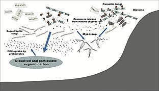  Roles of fungi in the marine carbon cycle

• 
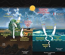  Carbon cycle
• 
  Carbon cycle
• 
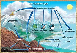  Carbon cycle
• 
  Ocean carbon cycle
• 
  Carbon cycle flux
• 
  Carbon sequestration
• 
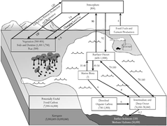  Climate change carbon cycle
• 
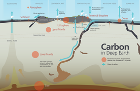  Reservoirs and fluxes of carbon in deep Earth
• 
  Carbon cycle-simple diagram
• 
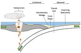  Subduction - accretionary
• 
  Subduction - Trench Schematic
• 
  Carbon dioxide emissions global carbon cycle

Microscale heterogeneity in the ocean and its potential impacts on the marine carbon cycle. Phytoplankton-bacterium interactions for example (depicted in the central droplet of seawater) might directly influence biogeochemical cycles, energy transfer to higher trophic levels, sequestration of refractory carbon, and release of climate-active gases.

Conceptual diagram of ice sheets in the global carbon cycle. The diagram indicates the potential direct and indirect impacts of ice sheets. (1) direct sequestration or emission of CO2/CH4 by microbial activity in ice sheets, (2) burial of terrestrial OM exported from ice sheets by rivers, (3) emission of CO2 by respiration or uptake by primary production in the oceans (4) export production–OM produced by primary production which is not recycled before it sinks to the ocean floor.

"The cycling of carbon on Earth exerts a fundamental influence upon the greenhouse gas content of the atmosphere, and hence global climate over millennia. Until recently, ice sheets were viewed as inert components of this cycle and largely disregarded in global models. Research in the past decade has transformed this view, demonstrating the existence of uniquely adapted microbial communities, high rates of biogeochemical/physical weathering in ice sheets and storage and cycling of organic carbon (>104 Pg C) and nutrients."

Stores and fluxes in present day ice sheets. A summary diagram indicating stores and fluxes of nutrients for present day ice sheets, and the predicted impact on CO2 (where data exists). The estimated size of carbon stores (Pg C) and Fluxes (Tg a−1).

Silica cycle

Marine and terrestrial contributions to the silica cycle are shown, with the relative movement (flux) provided in units of Tmol Si/yr. Marine biological production primarily comes from diatoms. Estuary biological production is due to sponges. Values of flux as published by Tréguer & De La Rocha. Reservoir size of silicate rocks, as discussed in the sources section, is 1.5x10²¹ Tmol.

From

Silica cycle...

Siliceous organisms in the ocean, such as diatoms and radiolaria, are the primary sink of dissolved silicic acid into opal silica. Once in the ocean, dissolved Si molecules are biologically recycled roughly 25 times before export and permanent deposition in marine sediments on the seafloor. This rapid recycling is dependent on the dissolution of silica in organic matter in the water column, followed by biological uptake in the photic zone. The estimated residence time of the silica biological reservoir is about 400 years. Opal silica is predominately undersaturated in the world's oceans. This undersaturation promotes rapid dissolution as a result of constant recycling and long residence times. The estimated turnover time of Si is 1.5x10⁴ years. The total net inputs and outputs of silica in the ocean are 9.4 ± 4.7 Tmol Si yr⁻¹ and 9.9 ± 7.3 Tmol Si yr⁻¹, respectively.

Biogenic silica production in the photic zone is estimated to be 240 ± 40 Tmol Si year ⁻¹. Dissolution in the surface removes roughly 135 Tmol Si year⁻¹, while the remaining Si is exported to the deep ocean within sinking particles. In the deep ocean, another 26.2 Tmol Si Year⁻¹ is dissolved before being deposited to the sediments as opal rain.  Over 90% of the silica here is dissolved, recycled and eventually upwelled for use again in the euphotic zone.

• 
  Silica cycle
• 
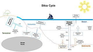
  Silica cycle
• 
  Forms of carbon in deep Earth
• 
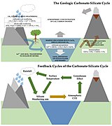  Carbon-Slicate Cycle Feedbacks

• Carbonate–silicate cycle

Oxygen cycle

See also: Oxygenation (environmental)

Annual mean sea surface dissolved oxygen for the World Ocean. Data from the World Ocean Atlas 2009.

• 
  Oxygen cycle
• 
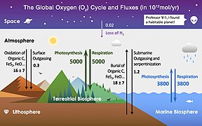  Oxygen cycle
• 
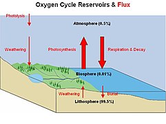  Oxygen cycle

• Limburg, K.E., Breitburg, D., Swaney, D.P. and Jacinto, G. (2020) "Ocean Deoxygenation: A Primer. One Earth", 2(1): 24–29. doi:10.1038/s41598-018-27793-4

Ocean ventilation and deoxygenation

Schematic of ventilation in an idealized high-latitude ocean basin. The basin extends from a high-latitude landmass (or, equivalently, the North Pole) to an arbitrary mid-latitude zonal boundary of length L. The basin contains n sloping isopycnal layers of (spatially and temporally variable) thickness h and meridional velocity v that outcrop into the upper-ocean mixed layer (of depth H) within the region. Like the real-world high-latitude oceans, the basin hosts a double-celled overturning circulation, with inflow in intermediate layers and outflow in surface and deep layers. Ventilation is quantified with a surface-sourced tracer C, which crosses the mixed layer base with vertical velocity w and at an integrated rate FC. The tracer has interior sources and sinks SC within the basin, and is exported through the mid-latitude boundary at a rate TC.

"Changes of ocean ventilation rates and deoxygenation are two of the less obvious but important indirect impacts expected as a result of climate change on the oceans. They are expected to occur because of (i) the effects of increased stratification on ocean circulation and hence its ventilation, due to reduced upwelling, deep-water formation and turbulent mixing, (ii) reduced oxygenation through decreased oxygen solubility at higher surface temperature, and (iii) the effects of warming on biological production, respiration and remineralization. The potential socio-economic consequences of reduced oxygen levels on fisheries and ecosystems may be far-reaching and significant... Our current understanding of both the causes and consequences of reduced oxygen in the ocean, and our ability to represent them in models are therefore inadequate, and the reasons for this remain unclear. It is too early to say whether or not the socio-economic consequences are likely to be serious. However, the consequences are ecologically, biogeochemically and climatically potentially very significant, and further research on these indirect impacts of climate change via reduced ventilation and oxygenation of the oceans should be accorded a high priority."

• Oxygen minimum zone
• Microbiology of oxygen minimum zones
• Watson, A.J., Lenton, T.M. and Mills, B.J. (2017) "Ocean deoxygenation, the global phosphorus cycle and the possibility of human-caused large-scale ocean anoxia". Philosophical Transactions of the Royal Society A: Mathematical, Physical and Engineering Sciences, 375: 20160318. doi:10.1098/rsta.2016.0318.

Chaotic nature of ocean ventilation

Schematic illustration of laminar (blue) and chaotic (red) ventilation pathways of adjacent particles on a density surface. The particles are adjacent at time t and the i^th particle left the mixed layer at time t-Δt_j.

Potential physical, ecological and biogeochemical mechanisms contributing to ocean deoxygenation in the Anthropocene

Nutrient cycles

Economic value of bivalve nutrient extraction. Linking processes to services to economic values. The arrows are illustrative and not a complete mapping of the interconnection between the different aspects.

Nutrient extraction services provided by bivalves. Blue mussels are used as examples but other bivalves like oysters can also provide these nutrient extraction services.

Seabird ornitheutrophication coupling. Schematic summary of processes coupling local and regional environmental effects in seabird colonies. Colonies can be considered as nutrient hot spots, especially, for N and P. Nitrogen is the key nutrient in marine environments and phosphorous in continental waters. Both are found in high concentrations in seabird feces. Uric acid is the dominant N compound, and during its mineralization different N forms are produced: (1) ammonification produces NH3 and NH4+, and (2) nitrification produces NO3− by NH4+ oxidation. Under the alkaline conditions, typical of the seabird feces, the NH3 is rapidly volatized (3) and transformed to NH4+, which is transported out of the colony, and through wet-deposition exported to distant ecosystems, which are eutrophized (4). Similarly, nutrients in the colony can be leached and transported out through runoff and groundwater seepage (5), generating in cases (4) and (5) environmental impacts at the regional level. On the other hand, NH4+ in soil (ornithogenic soils) can be adsorbed by organominerals and remain as an exchangeable cation (panel a). The soil NH4+ in the colony can be oxidized to nitrate through nitrification processes, and rapidly washed to subterranean or superficial waters, eutrophizing nearby ecosystems (local impact, 5). In both cases, the NO3− and NH4+ can reach creeks and small lakes, eutrophizing them (regional impact). Phosphorus cycle is simpler and has a rather reduced mobility. This element is found in a number of chemical forms in the seabird fecal material, but the most mobile and bioavailable is orthophosphate (HPO4=), which can be lixiviated (solubilized) to subterranean or superficial waters (5). However, an important fraction of the P can be adsorbed by Fe/Al oxyhydroxides in acidic soils. Through erosion, these colloids can reach anoxic freshwater or estuarine sediments, where P is liberated to the water column by the reductive dissolution of Fe(III) oxyhydroxides (panel b). If the colloids reach oxic marine sediments, P can still be liberated to the water by alkaline desorption (panel c), a process that involves changes in the surface charge of Fe/Al oxyhydroxides. In both cases, water eutrophization is produced.

Schematic model of nitrogen cycling in China’s aquaculture ecosystem. The unit is Tg N yr−1. The red lines represent Nr flow. The numbers in front of the parentheses represent the Nr flux in 2015; the numbers in parentheses represent the Nr flux in 1978. Only major flows are presented in this figure, but the flow description and data acquisition section in the methods section of this paper provide an overview of all simulated flows.

Cartoon representation of the proposed dust-bound Fe acquisition pathway employed mutually by Trichodesmium colonies and associated bacteria. a The N2-fixing marine cyanobacterium Trichodesmium spp., which commonly occurs in tropical and sub-tropical waters, is of large environmental significance in fertilizing the ocean with important nutrients. b Trichodesmium can establish massive blooms in nutrient poor ocean regions with high dust deposition, partly due to their unique ability to capture dust, center it, and subsequently dissolve it. c The current study explores biotic interactions within Trichodesmium colonies that lead to enhanced dissolution and acquisition of iron from dust. Bacteria residing within the colonies produce siderophores (c-I) that react with the dust particles in the colony core and generate dissolved Fe (c-II). This dissolved Fe, complexed by siderophores, is then acquired by both Trichodesmium and its resident bacteria (c-III), resulting in a mutual benefit to both partners of the consortium.

Nitrogen cycle

"Nitrogen (N) is a key element for life in the oceans. It controls primary productivity in many parts of the global ocean, consequently playing a crucial role in the uptake of atmospheric carbon dioxide. The marine N cycle is driven by multiple biogeochemical transformations mediated by microorganisms, including processes contributing to the marine fixed N pool (N2 fixation) and retained N pool (nitrification, assimilation, and dissimilatory nitrate reduction to ammonia), as well as processes contributing to the fixed N loss (denitrification, anaerobic ammonium oxidation and nitrite-dependent anaerobic methane oxidation). The N cycle maintains the functioning of marine ecosystems and will be a crucial component in how the ocean responds to global environmental change. In this review, we summarize the current understanding of the marine microbial N cycle, the ecology and distribution of the main functional players involved, and the main impacts of anthropogenic activities on the marine N cycle."

The main studied processes of the N cycle in different marine environments. Every coloured arrow represents a N transformation: N2 fixation (red), nitrification (light blue), nitrate reduction (violet), DNRA (magenta), denitrification (aquamarine), N-damo (green), and anammox (orange). Black curved arrows represent physical processes such as advection and diffusion.

Anthropogenic activities and their effects on the marine N cycling. Bioavailable N (Nb) is introduced into the marine ecosystems by runoff or atmospheric deposition, causing eutrophication, the formation of dead zones and the expansion of the ocean minimum zones (OMZs). The release of N oxides (N2O, NO) from anthropogenic activities and oxygen-depleted zones causes stratospheric ozone depletion leading to higher UVB exposition, which produces the damage of marine life, acid rain and ocean warming. Ocean warming causes water stratification, deoxygenation, and the formation of dead zones. Dead zones and OMZs are hotspots for anammox and denitrification, causing N loss (N2 and N2O). Elevated atmospheric CO2 acidifies seawater, decreasing pH-dependent N-cycling processes such as nitrification, and enhancing N2 fixation.

Nitrogen cycling in China’s aquaculture ecosystem. The unit is Tg N yr−1. The red lines represent Nr flow. The numbers in front of the parentheses represent the Nr flux in 2015; the numbers in parentheses represent the Nr flux in 1978.

• 
  Marine nitrogen cycle
• 
  Nitrogen cycle
• 

Phosphorus cycle

• 
  Phosphorus cycle

Sulfur cycle

• 
  Sulfur cycle
• 
  Sulfur cycle
• 
  Sulfur cycle
• 
  Sulfur cycle
• 
  Sulfur cycle

Water cycle

• 
  Water cycle
• 
• 
• 
  Water cycle [3]
• 
• 
• 
• 
• 
• 
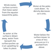
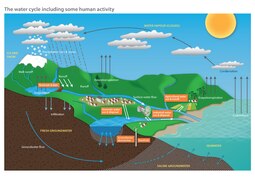
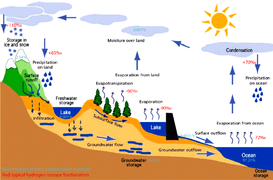  hydrological cycle

Rock cycle

• 
  Rock cycle in Wilson cycle
• 
  Rock cycle
• 
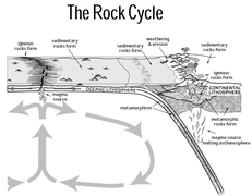
  Rock cycle
• 
  Rock cycle
• 
  Rock cycle

Mercury cycle

• Mercury cycle

Biogeochemical proxies

Schematic of atmospheric and oceanic sea ice proxies recorded in ice cores and marine sediments.

Temperature trends in different layers of the Southern Ocean

The layers are defined as main water masses of the Southern Ocean: Subtropical Water (TW), Mode Water (MW), Intermediate Water (IW), Circumpolar Deep Water (CDW), and Bottom Water (BW). Black arrows show the main overturning pathways in the basin, and the dashed black contours show a vertical slice of the deep-reaching Antarctic Circumpolar Current circulating clockwise around the Antarctic continent. The red arrows and associated numbers represent processes at play in the warming of the Southern Ocean and are discussed in the text: (1) increased surface stratification and shallowing of CDW layer, (2) increased heat uptake in the subpolar basins, (3) increased northward heat transport associated with increased subpolar heat uptake, (4) reduced eddy-​mediated southward heat transport across the Antarctic Circumpolar Current, (5) intrusion of CDW onto the continental shelves, and (6) warming of the bottom water ventilating the abyssal ocean.

used in paleoceanography

• google search

Global distribution of surface chlorophyll levels. Chlorophyll (a proxy for phytoplankton mass) is relatively low in the three HNLC regions (North Pacific, Equatorial Pacific, and Southern Ocean).

Role of microorganisms

"Microbial communities are key drivers of marine biogeochemistry. Our understanding of the incredible complexity and diversity of natural microbial populations has been greatly enhanced by the advent of cultivation-independent techniques for sequencing DNA directly from an environmental sample. Despite progress in describing the complexity of these natural systems, many gaps remain in our understanding of the distribution of genes and organisms in the oceans as well as the selective forces that structure community composition and distribution across space and time."

viruses

Intrinsic and extrinsic factors that can make viruses unsuccessful during their life cycle stages. Host specificity refers to the attachment and insertion of genetic material (DNA or RNA) into the hosts, latent period refers to the duration of the viral infection within the host during which virus particles are produced, burst size refers to the number of viral progeny released and particle state refers to the state where viruses are not within a host. Extrinsic factors are divided into host resistance mechanisms, abiotic and biotic stressors, and they can affect viruses during any of their life stages.

"Algal viruses are considered to be key players in structuring microbial communities and biogeochemical cycles due to their abundance and diversity within aquatic systems. Their high reproduction rates and short generation times make them extremely successful, often with immediate and strong effects for their hosts and thus in biological and abiotic environments. There are, however, conditions that decrease their reproduction rates and make them unsuccessful with no or little immediate effects. Here, we review the factors that lower viral success and divide them into intrinsic—when they are related to the life cycle traits of the virus—and extrinsic factors—when they are external to the virus and related to their environment. Identifying whether and how algal viruses adapt to disadvantageous conditions will allow us to better understand their role in aquatic systems. We propose important research directions such as experimental evolution or the resurrection of extinct viruses to disentangle the conditions that make them unsuccessful and the effects these have on their surroundings."

"Viruses are the most abundant life forms on Earth, with an estimated 1031 total viruses globally. The majority of these viruses infect microbes, whether bacteria, archaea or microeukaryotes. Given the importance of microbes in driving global biogeochemical cycles, it would seem, based on numerical abundances alone, that viruses also play an important role in the global cycling of carbon and nutrients. However, the importance of viruses in controlling host populations and ecosystem functions, such as the regeneration, storage and export of carbon and other nutrients, remains unresolved. Here, we report on advances in the study of ecological effects of viruses of microbes. In doing so, we focus on an area of increasing importance: the role that ocean viruses play in shaping microbial population sizes as well as in regenerating carbon and other nutrients... The study of viruses of microbes has undergone a revolution in the past 20 years. What has been termed "The Third Age of Phage" can be viewed more broadly as a renewal of interest in environmental viruses, and in particular in viruses of microbes [2-11]. This renewal has been spurred by advances in direct-imaging methods, sequencing technologies and bioinformatics that have revealed a previously unknown world of viral diversity in natural environments [12]. The study of viruses in the oceans has been key to many discoveries: from the finding that viruses have evolved novel lineages of key photosynthetic genes (as in cyanophages infecting Synechococcus and Prochlorococcus [13-17]) to the identification of many novel viral families that defy much of the conventional wisdom about viral life history (e.g. the discovery of “giant” algal-infecting viruses [18,19] and even viruses that exploit other viruses [20]). Altogether, it is well established that a diverse reservoir of viruses infect and lyse bacteria, archaea and microeukaryotes at the base of the ocean's food web [2,21]. Despite the growing literature on viruses of microbes, we remain relatively poorly informed concerning the dynamic, ecological effects of virus infection of marine microbes. In this report, we focus on the functional role of viruses within oceanic waters. In doing so, we highlight knowns, unknowns and challenges in three areas: (i) the role of ocean viruses in shaping microbial community composition; (ii) the role of ocean viruses in determining carbon and nutrient availability; (iii) modelling efforts to link viral infection of microbes with ecosystem-scale consequences."

"In marine environments, virus-mediated lysis of host cells leads to the release of cellular carbon and nutrients and is hypothesized to be a major driver of carbon recycling on a global scale. However, efforts to characterize the effects of viruses on nutrient cycles have overlooked the geochemical potential of the virus particles themselves, particularly with respect to their phosphorus content. In this Analysis article, we use a biophysical scaling model of intact virus particles that has been validated using sequence and structural information to quantify differences in the elemental stoichiometry of marine viruses compared with their microbial hosts. By extrapolating particle-scale estimates to the ecosystem scale, we propose that, under certain circumstances, marine virus populations could make an important contribution to the reservoir and cycling of oceanic phosphorus."

"Marine viruses have important roles in microbial mortality, gene transfer, metabolic reprogramming and biogeochemical cycling. In this Review, we discuss recent technological advances in marine virology including the use of near-quantitative, reproducible metagenomics for large-scale investigation of viral communities and the emergence of gene-based viral ecology. We also describe the reprogramming of microbially driven processes by viral metabolic genes, the identification of novel viruses using cultivation-dependent and cultivation-independent tools, and the potential for modelling studies to provide a framework for studying virus–host interactions. These transformative advances have set a rapid pace in exploring and predicting how marine viruses manipulate and respond to their environment."

"Viruses numerically dominate our oceans; however, we have only just begun to document the diversity, host range and infection dynamics of marine viruses, as well as the subsequent effects of infection on both host cell metabolism and oceanic biogeochemistry. Bacteriophages (that is, phages: viruses that infect bacteria) are highly abundant and are known to play critical roles in bacterial mortality, biogeochemical cycling and horizontal gene transfer. This Review Article summarizes current knowledge of marine viral ecology and highlights the importance of phage particles to the dissolved organic matter pool, as well as the complex interactions between phages and their bacterial hosts. We emphasize the newly recognized roles of phages as puppet masters of their bacterial hosts, where phages are capable of altering the metabolism of infected bacteria through the expression of auxiliary metabolic genes and the redirection of host gene expression patterns. Finally, we propose the ‘royal family model’ as a hypothesis to describe successional patterns of bacteria and phages over time in marine systems, where despite high richness and significant seasonal differences, only a small number of phages appear to continually dominate a given marine ecosystem. Although further testing is required, this model provides a framework for assessing the specificity and ecological consequences of phage–host dynamics."

• Middelboe, M. and Brussaard, C.P. (2017) "Marine viruses: Key players in marine ecosystems", Viruses, 9(10): 302;. doi:10.3390/v9100302. Material was copied from this source, which is available under a Creative Commons Attribution 4.0 International License.
• See Special Issue "Marine Viruses 2016"

"Viruses are a key component of marine ecosystems, but the assessment of their global role in regulating microbial communities and the flux of carbon is precluded by a paucity of data, particularly in the deep ocean. We assessed patterns in viral abundance and production and the role of viral lysis as a driver of prokaryote mortality, from surface to bathypelagic layers, across the tropical and subtropical oceans. Viral abundance showed significant differences between oceans in the epipelagic and mesopelagic, but not in the bathypelagic, and decreased with depth, with an average power-law scaling exponent of −1.03 km−1 from an average of 7.76 × 106 viruses ml−1 in the epipelagic to 0.62 × 106 viruses ml−1 in the bathypelagic layer with an average integrated (0 to 4000 m) viral stock of about 0.004 to 0.044 g C m−2, half of which is found below 775 m. Lysogenic viral production was higher than lytic viral production in surface waters, whereas the opposite was found in the bathypelagic, where prokaryotic mortality due to viruses was estimated to be 60 times higher than grazing. Free viruses had turnover times of 0.1 days in the bathypelagic, revealing that viruses in the bathypelagic are highly dynamic. On the basis of the rates of lysed prokaryotic cells, we estimated that viruses release 145 Gt C year−1 in the global tropical and subtropical oceans. The active viral processes reported here demonstrate the importance of viruses in the production of dissolved organic carbon in the dark ocean, a major pathway in carbon cycling."

"The encounter and capture of bacteria and phytoplankton by microbial predators and parasites is fundamental to marine ecosystem organization and activity. Here, we combined classic biophysical models with published laboratory measurements to infer functional traits, including encounter kernel and capture efficiency, for a wide range of marine viruses and microzooplankton grazers. Despite virus particles being orders of magnitude smaller than microzooplankton grazers, virus encounter kernels and adsorption rates were in many cases comparable in magnitude to grazer encounter kernel and clearance, pointing to Brownian motion as a highly effective method of transport for viruses. Inferred virus adsorption efficiency covered many orders of magnitude, but the median virus adsorption efficiency was between 5 and 25% depending on the assumed host swimming speed. Uncertainty on predator detection area and swimming speed prevented robust inference of grazer capture efficiency, but sensitivity analysis was used to identify bounds on unconstrained processes. These results provide a common functional trait framework for understanding marine host-virus and predator-prey interactions, and highlight the value of theory for interpreting measured life-history traits."

"Viruses are by far the most abundant entities in marine environments, and are mainly phages that infect bacteria and archaea, which also are a significant component of marine ecosystem and a major force behind marine biogeochemical cycles. As a major source of mortality, viral lysis can release highly labile cellular components, both organic matters and inorganic nutrients, regulating the metabolism of its hosts and influencing the biogeochemical cycles. During infection, viruses could hijack the metabolic system of hosts for its own propagation, thereby changing the metabolism and metabolites of host cells. This paper summarized the effects of viruses on the metabolism of marine bacterioplankton at both the cellular and community level, and its influence on the cycling of ocean elements. Then, the potential impact of environmental factors was assessed on the influence of viruses upon bacterial metabolism. This paper will contribute to a comprehensive understanding of the role of microbes within marine biogeochemical cycles."

bacteria

See also: Streamlining theory

"Little is still known of the impacts of protist grazing on bacterioplankton communities in the dark ocean. Furthermore, the accuracy of assessments of in situ microbial activities, including protist grazing, can be affected by sampling artifacts introduced during sample retrieval and downstream manipulations. Potential artifacts may be increased when working with deep-sea samples or samples from chemically unique water columns such as oxygen minimum zones (OMZs). OMZs are oxygen-depleted regions in the ocean, where oxygen concentrations can drop to <20 μM. These regions are typically located near eastern boundary upwelling systems and currently occur in waters occupying below about 8% of total ocean surface area, representing ~1% of the ocean's volume. OMZs have a profound impact not only on the distribution of marine Metazoa, but also on the composition and activities of microbial communities at the base of marine food webs. Here we present an overview of current knowledge of protist phagotrophy below the photic zone, emphasizing studies of oxygen-depleted waters and presenting results of the first attempt to implement new technology for conducting these incubation studies completely in situ (the Microbial Sampling- Submersible Incubation Device, MS-SID). We performed 24-h incubation experiments in the Eastern Tropical South Pacific (ETSP) OMZ. This preliminary study shows that up to 28% of bacterial biomass may be consumed by protists in waters where oxygen concentrations were down to ~4.8 μM and up to 13% at a station with nitrite accumulation where oxygen concentrations were undetectable. Results also show that shipboard measurements of grazing rates were lower than rates measured from the same water using the MS-SID, suggesting that in situ experiments help to minimize artifacts that may be introduced when conducting incubation studies using waters collected from below the photic zone, particularly from oxygen-depleted regions of the water column."

"Prochlorococcus and SAR11 are among the smallest and most abundant organisms on Earth. With a combined global population of about 2.7 × 1028 cells, they numerically dominate bacterioplankton communities in oligotrophic ocean gyres and yet they have never been grown together in vitro. Here we describe co-cultures of Prochlorococcus and SAR11 isolates representing both high- and low-light adapted clades. We examined: (1) the influence of Prochlorococcus on the growth of SAR11 and vice-versa, (2) whether Prochlorococcus can meet specific nutrient requirements of SAR11, and (3) how co-culture dynamics vary when Prochlorococcus is grown with SAR11 compared with sympatric copiotrophic bacteria. SAR11 grew 15–70% faster in co-culture with Prochlorococcus, while the growth of the latter was unaffected. When Prochlorococcus populations entered stationary phase, this commensal relationship rapidly became amensal, as SAR11 abundances decreased dramatically. In parallel experiments with copiotrophic bacteria; however, the heterotrophic partner increased in abundance as Prochlorococcus densities leveled off. The presence of Prochlorococcus was able to meet SAR11’s central requirement for organic carbon, but not reduced sulfur. Prochlorococcus strain MIT9313, but not MED4, could meet the unique glycine requirement of SAR11, which could be due to the production and release of glycine betaine by MIT9313, as supported by comparative genomic evidence. Our findings also suggest, but do not confirm, that Prochlorococcus MIT9313 may compete with SAR11 for the uptake of 3-dimethylsulfoniopropionate (DMSP). To give our results an ecological context, we assessed the relative contribution of Prochlorococcus and SAR11 genome equivalents to those of identifiable bacteria and archaea in over 800 marine metagenomes. At many locations, more than half of the identifiable genome equivalents in the euphotic zone belonged to Prochlorococcus and SAR11 – highlighting the biogeochemical potential of these two groups."

"As the smallest and most abundant primary producer in the oceans, the cyanobacterium Prochlorococcus is of interest to diverse branches of science. For the past 30 years, research on this minimal phototroph has led to a growing understanding of biological organization across multiple scales, from the genome to the global ocean ecosystem. Progress in understanding drivers of its diversity and ecology, as well as molecular mechanisms underpinning its streamlined simplicity, has been hampered by the inability to manipulate these cells genetically. Multiple attempts have been made to develop an efficient genetic transformation method for Prochlorococcus over the years; all have been unsuccessful to date, despite some success with their close relative, Synechococcus... Prochlorococcus is the most abundant cyanobacterium worldwide, dominating vast regions of the global oceans [19]. It may account for up to 50 % of the chlorophyll in oligotrophic ocean regions [20, 21] and is responsible for around 8.5 % of global ocean primary productivity [19]. Our understanding of Prochlorococcus biology and ecology has been greatly facilitated by the rise of metagenomic, metatranscriptomic, and metaproteomic studies of ocean samples over the past decade [22–26]. Because of its high relative abundance, it often dominates databases derived from surface microbial communities in the oceans [27], and has emerged as one of the best-described marine microorganisms with more than one thousand complete or nearly complete genomes available [28–30]. Prochlorococcus is a perfect example of the imbalance between the availability of genomic data and the dearth of genetic tools. Prochlorococcus’ numerical dominance in oligotrophic oceans is attributed to its small size (hence high surface/volume ratio), which enhances its ability to compete for limiting nutrients [31], and its vast genomic diversity [32–37], which expands the niche dimensions of the Prochlorococcus meta-population [28, 38, 39]."

archaea

"Archaea are ubiquitous and abundant members of the marine plankton. Once thought of as rare organisms found in exotic extremes of temperature, pressure, or salinity, archaea are now known in nearly every marine environment. Though frequently referred to collectively, the planktonic archaea actually comprise four major phylogenetic groups, each with its own distinct physiology and ecology. Only one group—the marine Thaumarchaeota—has cultivated representatives, making marine archaea an attractive focus point for the latest developments in cultivation-independent molecular methods. Here, we review the ecology, physiology, and biogeochemical impact of the four archaeal groups using recent insights from cultures and large-scale environmental sequencing studies. We highlight key gaps in our knowledge about the ecological roles of marine archaea in carbon flow and food web interactions. We emphasize the incredible uncultivated diversity within each of the four groups, suggesting there is much more to be done."

"Archaea constitute a considerable fraction of the microbial biomass on Earth. Like Bacteria they have evolved a variety of energy metabolisms using organic and/or inorganic electron donors and acceptors, and many of them are able to fix carbon from inorganic sources. Archaea thus play crucial roles in the Earth's global geochemical cycles and influence greenhouse gas emissions. Methanogenesis and anaerobic methane oxidation are important steps in the carbon cycle; both are performed exclusively by anaerobic archaea. Oxidation of ammonia to nitrite is performed by Thaumarchaeota. They represent the only archaeal group that resides in large numbers in the global aerobic terrestrial and marine environments on Earth. Sulfur-dependent archaea are confined mostly to hot environments, but metal leaching by acidophiles and reduction of sulfate by anaerobic, nonthermophilic methane oxidizers have a potential impact on the environment. The metabolisms of a large number of archaea, in particular those dominating the subsurface, remain to be explored."

protists

"Protists are microscopic eukaryotic microbes that are ubiquitous, diverse, and major participants in oceanic food webs and in marine biogeochemical cycles. The study and characterization of protists has a long and distinguished tradition. Even with this history, the extraordinary species diversity and variety of interactions of protists in the sea are only now being fully appreciated. Figure 1 shows representative examples of marine protists, and of methods used to visualize these microbes. Protists can be autotrophic or heterotrophic. The former, also called microscopic algae, contain chloroplasts, thrive by photosynthesis, and are at the base of all oceanic food webs, with the exception of deep-sea chemosynthetic ecosystems. There is a general trend for > 20-µm sized phytoplankton (microplankton), such as diatoms and dinoflagellates, to dominate episodically in coastal waters, while in the open ocean 2–20-µm sized cells (nanoplankton), such as coccolithophorids, sporadically form massive blooms that can be seen from space. However, during nonbloom seasons, even smaller cells (picoplankton—prokaryotes and eukaryotes less than a few micrometers in size) typically dominate phytoplankton biomass and production (Li, 2002; Worden et al., 2004). Some genera of marine picoalgae can “bloom” to very high concentrations (> 105 cells ml-1), Ostreococcus (Countway and Caron, 2006), while others are ubiquitous, such as Micromonas, which is found from arctic to tropical waters (Not et al., 2004; Worden, 2006)."

planktonic fungus

"Fungal contributions to ecosystem processes are well documented for terrestrial systems yet oceans, which account for most of the Earth’s surface, have remained poorly explored with regards to organisms in this kingdom. Here, we demonstrate that, although in low relative abundance (i.e., fungal reads made up 1.4–2.9% of the metagenomes), fungi contribute to both phylogenetic and functional microbial diversity with a conserved fungal presence in global marine samples. Universally distributed taxa and functions implicate them in complex carbon and fatty acid metabolism, with depth stratification along pelagic zones. Functional differences in observed genes between epipelagic and mesopelagic waters indicate changes in UV protection, shift to carbohydrate limited diets, as well as alternative energy sources. Metagenomic data also provided evidence for a latitudinal gradient in fungal diversity linked to temperature shifts. Our results suggest that fungi contribute to multiple biogeochemical cycles in the pelagic ocean, and could be integral for ecosystem functioning through provision of key nutrients."

"Growing interest in understanding the relevance of marine fungi to food webs, biogeochemical cycling, and biological patterns necessitates establishing a context for interpreting future findings. To help establish this context, we summarize the diversity of cultured and observed marine planktonic fungi from across the world. While exploring this diversity, we discovered that only half of the known marine fungal species have a publicly available DNA locus, which we hypothesize will likely hinder accurate high-throughput sequencing classification in the future, as it does currently. Still, we reprocessed >600 high-throughput datasets and analyzed 4.9 × 109 sequences (4.8 × 109 shotgun metagenomic reads and 1.0 × 108 amplicon sequences) and found that every fungal phylum is represented in the global marine planktonic mycobiome; however, this mycobiome is generally predominated by three phyla: the Ascomycota, Basidiomycota, and Chytridiomycota. We hypothesize that these three clades are the most abundant due to a combination of evolutionary histories, as well as physical processes that aid in their dispersal. We found that environments with atypical salinity regimes (>5 standard deviations from the global mean: Red Sea, Baltic Sea, sea ice) hosted higher proportions of the Chytridiomycota, relative to open oceans that are dominated by Dikarya. The Baltic Sea and Mediterranean Sea had the highest fungal richness of all areas explored. An analysis of similarity identified significant differences between oceanographic regions. There were no latitudinal gradients of marine fungal richness and diversity observed. As more high-throughput sequencing data become available, expanding the collection of reference loci and genomes will be essential to understanding the ecology of marine fungi."

phytoplankton

(A) Size distribution of virus, bacteria, and grazers

Virus radius relates to capsid cross-section, and bacteria and grazer values are equivalent spherical radius. Viruses include a compilation of bacteriophage, and viruses of eukaryotic algae, including giant viruses. A compilation of grazers are included and a compilation of bacteria that includes both marine and non-marine species. Frequency at each size represents the number of cultured strains, which says nothing of the relative abundance at each size, or phylogenetic contrast.

(B) Contrasting strategies to encounter prey

Represented here with the green circle. Viruses are dependent on Brownian motion, whereas grazers must swim to find prey.

"Carbon, nitrogen and phosphorus are essential elements required for all life on Earth. In the marine environment, dissolved inorganic carbon, nitrogen and phosphorus are utilized during phytoplankton growth to form organic material, which is respired and remineralized back to inorganic forms by the activity of bacteria, Archaea and zooplankton. The net result of the photosynthesis, calcification and respiration of marine plankton is the uptake of carbon dioxide (CO2) from the atmosphere, its sequestration to the deep ocean as organic and inorganic carbon and its availability to fuel all fish and shellfish production. The cycling of carbon by marine plankton is inextricably linked to that of nitrogen and phosphorus; thus marine plankton mediate climate through influencing the atmospheric concentration of not only CO2, but also nitrous oxide (N2O). Increasing anthropogenically derived atmospheric CO2 concentrations impact plankton mediated biogeochemical cycles through increasing seawater temperature and dissolution of CO2, leading to changes in water column mixing, availability of light and nutrients, decreasing dissolved oxygen and changing carbonate chemistry. This chapter describes how the activity of phytoplankton, bacteria and Archaea drive the marine biogeochemical cycles of carbon, nitrogen and phosphorus, and how climate driven changes in plankton abundance and community composition are influencing these biogeochemical cycles in the North Atlantic Ocean and adjacent seas."

zooplankton

"Exploring climate and anthropogenic impacts on marine ecosystems requires an understanding of how trophic components interact. However, integrative end-to-end ecosystem studies (experimental and/or modelling) are rare. Experimental investigations often concentrate on a particular group or individual species within a trophic level, while tropho-dynamic field studies typically employ either a bottom-up approach concentrating on the phytoplankton community or a top-down approach concentrating on the fish community. Likewise the emphasis within modelling studies is usually placed upon phytoplankton-dominated biogeochemistry or on aspects of fisheries regulation. In consequence the roles of zooplankton communities (protists and metazoans) linking phytoplankton and fish communities are typically under-represented if not (especially in fisheries models) ignored. Where represented in ecosystem models, zooplankton are usually incorporated in an extremely simplistic fashion, using empirical descriptions merging various interacting physiological functions governing zooplankton growth and development, and thence ignoring physiological feedback mechanisms. Here we demonstrate, within a modelled plankton food-web system, how trophic dynamics are sensitive to small changes in parameter values describing zooplankton vital rates and thus the importance of using appropriate zooplankton descriptors. Through a comprehensive review, we reveal the mismatch between empirical understanding and modelling activities identifying important issues that warrant further experimental and modelling investigation. These include: food selectivity, kinetics of prey consumption and interactions with assimilation and growth, form of voided material, mortality rates at different age-stages relative to prior nutrient history. In particular there is a need for dynamic data series in which predator and prey of known nutrient history are studied interacting under varied pH and temperature regimes."

• Everett, J.D., Baird, M.E., Buchanan, P., Bulman, C., Davies, C., Downie, R., Griffiths, C., Heneghan, R., Kloser, R.J., Laiolo, L. and Lara-Lopez, A. (2017) "Modeling what we sample and sampling what we model: challenges for zooplankton model assessment". Frontiers in Marine Science, 4: 77. doi:10.3389/fmars.2017.00077. Material was copied from this source, which is available under a Creative Commons Attribution 4.0 International License.

Classic food web and the microbial loop

Conceptual model of marine food web

P: phytoplankton, Z: zooplankton, N: nutrients, M: mixotroph, B: bacteria, D: detritus, HTL: higher trophic levels
solid arrows: inputs; dashed arrows: outputs; blue arrows: mixing; red and green arrows: exchange between the mixed surface layer and lower water

Azam's paper...

• Azam, F., T. Fenchel, J.G. Field, J.S. Gray, L.A. Meyer-Reil, and F. Thingstad (1983) [www.jstor.org/stable/24814647 "The ecological role of water-column microbes in the sea"]. Marine Ecology Progress Series, 10: 257-263.

On the "classic" food web (though he doesn't use the word "classic") and the microbial loop.

"Prior to the 1980s, the structure of the ecosystem in the pelagic marine waters was typically described through what is now termed the “classical” food web (Steele, 1974, Cushing, 1975). Within this structure, primary production is attributed to photoautotrophic phytoplankton. These phytoplankton are then consumed by the “herbivorous” zooplankton (i.e., primary consumers) which are in turn ingested by carnivorous zooplankton and pelagic fish, which then serve as food for larger fish. Despite some earlier suggestions to modify this classic food web structure (e.g., Pomeroy, 1974), it was not until the early 1980s that the importance of microbial production gained recognition (Williams, 1981, Fenchel, 1982), and the planktonic food web concept was broadened towards a more integrated view (the microbial food web). In this new defined structure phytoplankton as well as bacteria are consumed by protozoan grazers (Sherr and Sherr, 1994, Calbet, 2008), thus providing an additional food source for copepods and higher trophic levels. Following such studies, Azam et al. (1983) proposed the “microbial loop” as an addition to the food web, within which dissolved organic carbon (DOC) is reincorporated into the food web, mediated by microbial activity."

- mixotrophic

Gifford's paper:

• Gifford, D.J. (1991) "The protozoan‐metazoan trophic link in pelagic ecosystems". The Journal of Protozoology, 38(1): 81–86. doi:10.1111/j.1550-7408.1991.tb04806.x.

"The recognition of the importance of the microbial loop led to the “link-sink” debate (Gifford, 1991), questioning whether the activity of the protozoan grazers served as a “link” between the microbial loop and the classical food chain (Sanders and Porter, 1987), or as a “sink” for carbon (Ducklow et al., 1986). Various field studies, experimental results and modelling efforts have subsequently shown microzooplankton to be a link between the classical and microbial food webs in marine as well as fresh water bodies thus acting as conduits of energy and nutrients between the microbial level and higher trophic levels (Suttle et al., 1986, Frost, 1987, Cushing, 1995, Calbet and Saiz, 2005). Additionally, based on stoichiometric and biochemical grounds, microzooplankton, rather than phytoplankton, could be expected to be better prey for mesozooplankton (Klein Breteler et al., 1999, Broglio et al., 2003, Mitra and Flynn, 2005). The latest twist to this is the concept that much of the plankton community currently split between either phototrophic phytoplankton or heterotrophic microzooplankton should be recognised as mixotrophic (Flynn et al., 2013, Mitra et al., 2014)".

- mathematical descriptions

"Today, the construction, testing and deployment of mathematical descriptions of plankton dynamics are central planks in marine ecology and climate change research. Many of these studies are based on the classic ecosystem model of Fasham et al. (1990), or variations on that theme. However, while over the last half century our understanding of aquatic ecology has undergone a substantial change, models portraying these systems have not developed in line with field and laboratory observations. Model structure and complexity has not typically changed in ecosystem models to reflect improvements in our understanding of biological complexity with its attendant feedback mechanisms (Mitra and Davis, 2010, Rose et al., 2010). The dramatic increase in model complexity over this period has been almost wholly focussed on the phytoplankton–nutrient link, with regard to variables, processes and parameters. Very little, by comparison, has been done with the Z component, quite often employing only 2 classes (e.g., 78 P boxes vs. 2 Z boxes in Follows et al., 2007). Despite the plethora of mechanistic zooplankton models which have been developed over the past two decades (e.g., Carlotti and Hirche, 1997, Carlotti and Wolf, 1998, Mitra, 2006, Mitra and Flynn, 2007, Flynn and Irigoien, 2009), the Z-boxes within ecosystem models are still biologically extremely simplistic with little or no differences in the physiological descriptions between the different Z-boxes. This is despite the manifest difference in the ecophysiology of the protist microzooplankton and the metazoan zooplankton. Increased complexity has usually been in numerical rather than detailed structural complexity; for example, 1-box representing the entire zooplankton (Z) community vs. 3-boxes representing different zooplankton functional types (e.g., Franks, 2002 vs. Blackford et al., 2004)."

- top down/bottom up

"The zooplankton community has thus been typically side-lined within ecosystem studies, not receiving the same level of importance as the phytoplankton and fish communities. Within biogeochemical models, zooplankton represent the top trophic level acting as a closure function, while within many fisheries models, zooplankton form the bottom level (see reviews by Plagányi, 2007, Carlotti and Poggiale, 2010, Fulton, 2010). However, there is a growing recognition of the need to bring together these two strands of research (biogeochemical and fisheries) through development of end-to-end ecosystem models combining physicochemical oceanographic descriptors with the biology of all trophic levels from microbes to higher-trophic-level, including humans, in a single modelling framework (Mitra and Davis, 2010, Rose et al., 2010). Fig. 1 presents a conceptual model of such an end-to-end food web ecosystem. The zooplankton community (Z) acts as the conduit for the transfer of energy and material from the primary producers to the higher trophic levels and has a pivotal role in recycling and export of nutrients. Thus the zooplankton community is the critical link between biogeochemistry and fisheries (Carlotti and Poggiale, 2010, Mitra and Davis, 2010).

inverted pyramids

Comparison of ecosystem structure shape between model and results from Palmyra Atoll. Width of each rectangle shows the relative biomass of each trophic level.

Palmyra Atoll

Grey reef shark

Relationship between ecosystem structure and size-spectrum scaling. Width of bars represent relative abundance or biomass for value of the mass scaling exponent, k. Gray shading based on the distributions of k for marine ecosystems based on empirical estimates of trophic efficiency (TE) and predator:prey mass ratios (PPMR). Arrows denote flow of energy and hold for all pyramids. Trophic compartment (level) is given on right.

Higher trophic level fish, like this blacktip reef shark, can have a high relative biomass on coral reefs

mineral dust

Nutrients in the dust

"One of the major sources of essential nutrients to the ocean is mineral dust, which can deposit nitrogen, phosphorus, and iron, a biologically-important trace metal, into the open ocean, making mineral dust deposition an important factor controlling phytoplankton growth. The Saharan and Gobi Deserts are major sources of mineral dusts, which can be transported from source areas over thousands of kilometers. Climate change models forecast increased levels of dust deposition on the open ocean, and so the study here set out to understand how dust additions impact diatom growth."[8]

trace elements

"Trace elements serve important roles as regulators of ocean processes including marine ecosystem dynamics and carbon cycling. The role of iron, for instance, is well known as a limiting micronutrient in the surface ocean. Several other trace elements also play crucial roles in ecosystem function and their supply therefore controls the structure, and possibly the productivity, of marine ecosystems. Understanding the biogeochemical cycling of these micronutrients requires knowledge of their diverse sources and sinks, as well as their transport and chemical form in the ocean. Much of what is known about past ocean conditions, and therefore about the processes driving global climate change, is derived from trace-element and isotope patterns recorded in marine deposits. Reading the geochemical information archived in marine sediments informs us about past changes in fundamental ocean conditions such as temperature, salinity, pH, carbon chemistry, ocean circulation and biological productivity. These records provide our principal source of information about the ocean’s role in past climate change. Understanding this role offers unique insights into the future consequences of global change. The cycle of many trace elements and isotopes has been significantly impacted by human activity. Some of these are harmful to the natural and human environment due to their toxicity and/or radioactivity. Understanding the processes that control the transport and fate of these contaminants is an important aspect of protecting the ocean environment. Such understanding requires accurate knowledge of the natural biogeochemical cycling of these elements so that changes due to human activity can be put in context".

Biomass composition

"Obtaining a quantitative global picture of life in the great expanses of the oceans is a challenging task. By integrating data from across existing literature, we provide a comprehensive view of the distribution of marine biomass between taxonomic groups, modes of life, and habitats."

Schematic representation of the fate of DOM in the ocean. Arrows indicate the various production (arrowhead pointing toward DOM pool) and removal processes of DOM (arrowhead pointing away), while the dashed arrows represent dominant biological processes involved in the transfer of DOM. Due to these processes, the fraction of labile DOM decreases rapidly with depth, whereas the refractory character of the DOM pool considerably increases during its export to the deep ocean. DOM, dissolved organic matter.

Overview of the role of phytoplankton on various compartments of the marine environment including the atmospheric gas composition, inorganic nutrients, and trace element fluxes as well as the transfer and cycling of organic matter via biological processes. The photosynthetically fixed carbon is rapidly recycled and reused in the surface ocean, while a certain fraction of this biomass is exported as sinking particles to the deep ocean, where it is subject to ongoing transformation processes, e.g., remineralization.

Modeling biological oceanography

Example of a regional ocean model

This example is used to simulate lower trophic level processes throughout the Bering Sea. In the schematic, circular nodes represent state variables (gold indicates nutrient, green indicates producer, blue indicates consumer, brown indicates detritus). Edges (lines) represent fluxes between state variables and curve clockwise from source node to sink node. Edge colors indicate process type: green indicates primary production, blue indicates grazing and predation, brown indicates egestion, gold indicates respiration, red indicates remineralization, pink indicates nitrification, orange indicates non-predatory mortality, tan indicates excretion, purple indicates convective exchange, gray indicates sinking to seafloor, and navy indicates freezing/melting of ice.

–––––––––––––––––––––––––––––––––––––––––––––––––––––––––––––
The example model is the Bering Ecosystem Study Nutrient-Phytoplankton-Zooplankton model (BESTNPZ)

• Marine biogeochemical models
• Marine food web models

"Nearly 100 years ago, Alfred Lotka published two short but insightful papers describing how ecosystems may organize. Principally, Lotka argued that ecosystems will grow in size and that their cycles will spin faster via predation and nutrient recycling so as to capture all available energy, and that evolution and natural selection are the mechanisms by which this occurs and progresses. Lotka's ideas have often been associated with the maximum power principle, but they are more consistent with recent developments in nonequilibrium thermodynamics, which assert that complex systems will organize toward maximum entropy production (MEP). In this review, we explore Lotka's hypothesis within the context of the MEP principle, as well as how this principle can be used to improve aquatic biogeochemistry models. We need to develop the equivalent of a climate model, as opposed to a weather model, to understand marine biogeochemistry on longer timescales, and adoption of the MEP principle can help create such models."

"In current process-based biogeochemical models, mathematical expressions derived from available theoretical or empirical relationships are used to define the interactions between numerous state variables. The parameterization of these approximate mathematical expressions relies mainly on maximizing agreement between simulations and observations. These models are highly nonlinear, location-specific, and challenging to scale or apply in a different environment. The Maximum Energy Production (MEP) modelling approach presented here is based on the hypothesis that living systems evolve and organize to maximize free energy dissipation over the greatest possible spatial and temporal scales. In this study, we used a trait-based global ocean modeling system (MITgcm Darwin) to calculate entropy fluxes among different biotic constituents in the euphotic zone. Reaction free energies associated with different metabolic functions in a biological system, such as growth, nutrient uptake, nitrogen fixation, and denitrification, were calculated using simplified stoichiometric equations and reaction rates derived from the model for simple and complex food web structures. The preliminary results suggest that maximum entropy production can be used as a criterion to select food web configurations that may better represent natural marine ecosystems."

FROM Alfred J. Lotka... His earlier work was centered on energetics and applications of thermodynamics in life sciences. Lotka proposed the theory that the Darwinian concept of natural selection could be quantified as a physical law. The law that he proposed was that the selective principle of evolution was one which favoured the maximum useful energy flow transformation. The general systems ecologist Howard T. Odum later applied Lotka's proposal as a central guiding feature of his work in ecosystem ecology. Odum called Lotka's law the maximum power principle.

For the drama of life is like a puppet show in which stage, scenery, actors and all are made of the same stuff... and if we would catch the spirit of the piece, our attention must not be absorbed in the characters alone, but must be extended also to the scene, of which they are born, on which they play their part, and with which, in a little while, they merge again

— Alfred Lotka (1925)

For the drama of life is like a puppet show in which stage, scenery, actors and all are made of the same stuff... and if we would catch the spirit of the piece, our attention must not be absorbed in the characters alone, but must be extended also to the scene, of which they are born, on which they play their part, and with which, in a little while, they merge again – Alfred Lotka (1925)

• What did Lotka really say?
• How reliable are ocean models?
• Raäisaänen, J. (2007) "How reliable are climate models?". Tellus A: Dynamic Meteorology and Oceanography, 59(1): 2–29. doi:10.1111/j.1600-0870.2006.00211.x.
• How reliable are climate models?, Skeptical Science.
• Smith, Ryan & Kelly, Jonathan & Nazarzadeh, Kimia & Sukhatme, Gaurav. (2013). An Investigation on the Accuracy of Regional Ocean Models Through Field Trials. Proceedings - IEEE International Conference on Robotics and Automation. 10.1109/ICRA.2013.6631057.
• Ocean general circulation model

Marine sediments

Size spectra of marine communities and sources of sinking particles. The lines show idealized responses of community size spectra to changes in fish abundance. Because the abundance of organisms generally decreases with size, zooplankton will produce large amounts of more slowly-sinking faecal pellets, while large fish will produce small amounts of rapidly-sinking fecal pellets. The hypothetical predator-removal spectra are inspired by the simulated impacts of fishing on size spectrum models.

Fish populations are linked to ocean biogeochemistry by their reliance on primary production for food, and dissolved oxygen to breathe. It is also possible that marine fish modify biogeochemical dynamics, as do freshwater fish, through top-down trophic cascades, but there has been relatively little consideration of this possibility. This lack of consideration may reflect a lack of importance; alternatively, it may simply reflect the lack of appropriate observations with which to constrain such relationships. Here, we draw attention to the potential use of marine sediments as long-term simultaneous monitors of both fish abundance and marine biogeochemical dynamics. We compile published sediment proxy records of fish abundance from the west coasts of the Americas, and compare them with biogeochemical climatic signals, we find a small number of statistically significant relationships between fish debris and biogeochemical variables, at least some of which are likely to reflect causal relationships. Considering total organic carbon(TOC), the most commonly-measured biogeochemical variable, some positive correlations with fish abundance are found, consistent with bottom-up control of fish abundance by primary production, or a planktivore-herbivore-phytoplankton trophic cascade. Negative correlations are also found, which could reflect sedimentary processes, the influence of upwelling-driven oxygen and nutrient dynamics on primary production and fish populations, and/or impacts of fish stocks on carbon fluxes by altering the recycling of carbon within the water column. Although the number of available measurements is too small to draw strong conclusions, the results point to plausible cases of bottom-up forcing, trophic cascades, and influence of dissolved oxygen concentrations on fish habitat.

Benthic foraminifera

Relation between pore surface area on the penultimate and antepenultimate chambers of eipfaunal foraminifera and dissolved oxygen concentration in of ambient bottom waters. Large dots represent average values of specimens collected alive at each location; smaller dots represent individual values of specimen chambers. Lines with bars represent standard deviations.

• Schmiedl, G. (2019) "Use of Foraminifera in Climate Science". In: Oxford Research Encyclopedia of Climate Science: Past Climates. doi:10.1093/acrefore/9780190228620.013.735.

Anthropogenic changes

"The prokaryotic and eukaryotic microorganisms that drive the pelagic ocean's biogeochemical cycles are currently facing an unprecedented set of comprehensive anthropogenic changes. Nearly every important control on marine microbial physiology is currently in flux, including seawater pH, pCO2, temperature, redox chemistry, irradiance and nutrient availability. Here, we examine how microorganisms with key roles in the ocean carbon and nitrogen cycles may respond to these changes in the Earth's largest ecosystem. Some functional groups such as nitrogen-fixing cyanobacteria and denitrifiers may be net beneficiaries of these changes, while others such as calcifiers and nitrifiers may be negatively impacted. Other groups, such as heterotrophic bacteria, may be relatively resilient to changing conditions. The challenge for marine microbiologists will be to predict how these divergent future responses of marine microorganisms to complex multiple variable interactions will be expressed through changing biogeography, community structure and adaptive evolution, and ultimately through large-scale alterations of the ocean's carbon and nutrient cycles."

Overview about climatic changes and their effects on the ocean after Ciais et al. (2013) and Rhein et al. (2013). Regional effects are displayed in italics. Excess solar radiation enters the atmosphere. Ice reflects this radiation, but it is taken up by the surface ocean, leading to its warming. Ocean warming results in land ice melt and thermal expansion, which both result in a sea level rise. Heating of vast areas of the surface ocean also slowly heats up the intermediate water layer which, among others, can ultimately lead to regional changes of deep water. Regional freshening occurs on sites with melting land ice. Regional salinification on the contrary happens in areas of vast evaporation. Surface ocean warming also decreases the solubility of gases, leading to a reduced oxygen concentration and thus changes in the sea-oxygen flux. Excess anthropogenic carbon dioxide enhances its uptake by the ocean and leads to a gradual acidification of the ocean. A decreasing pH results in bicarbonate undersaturation, which causes dissolving of shells and other minerals. Regional input of reactive nitrogen can lead to fertilization and eutrophication. Another regional effect is the occurrence of high waves. Heating, reduced oxygen concentrations and eutrophication lead to higher stratification of water masses.

megafauna

"In a paper published in Science Advances, an international team of researchers have examined traits of marine megafauna species to better understand the potential ecological consequences of their extinction under different future scenarios. Defined as the largest animals in the oceans, with a body mass that exceeds 45kg, examples include sharks, whales, seals and sea turtles. These species serve key roles in ecosystems, including the consumption of large amounts of biomass, transporting nutrients across habitats, connecting ocean ecosystems, and physically modifying habitats."

"Habitat loss is accelerating a global extinction crisis. Conservation requires understanding links between species and habitats. Emerging research is revealing important associations between vegetated coastal wetlands and marine megafauna, such as cetaceans, sea turtles, and sharks. But these links have not been reviewed and the importance of these globally declining habitats is undervalued. Here, we identify associations for 102 marine megafauna species that utilize these habitats, increasing the number of species with associations based on current International Union for the Conservation of Nature (IUCN) species assessments by 59% to 174, accounting for over 13% of all marine megafauna. We conclude that coastal wetlands require greater protection to support marine megafauna, and present a simple, effective framework to improve the inclusion of habitat associations within species assessments."

---

references

The 100 µm length scale in the microbial ocean

The 100 µm length scale in the microbial ocean

100 µm is a useful yardstick in the microscale world of marine bacteria. While environmental processes affecting microbial ecology often unfold at larger scales, as exemplified by the phytoplankton bloom depicted in blue hues in the background, it is the microscale that most immediately affects the life of marine and aquatic bacteria. Characteristic distances among bacteria, whether motile (flagellated cells) or non-motile (circular, non-flagellated cells), as well as between microbes and viruses occur over scales on the order of 100 µm, here denoted as ‘O(100 µm)’. So, too, do gradients of dissolved organic matter (yellow-green coloration and grey contour lines) emanating for example from phytoplankton (diatom on the top right), to which motile bacteria can respond by directional swimming (thick dashed trajectory). Processes such as turbulence (not depicted) also contribute to spatial heterogeneity at O(100 µm) scales, further increasing the prominence of this scale in microbial ecology.

Turbulent stirring and molecular diffusion

"100 µm is a fundamental scale for chemical gradients that bacteria experience in the ocean even when sources are larger than 100 µm, because of turbulent stirring, which can rapidly create filaments and sheets of O(100 µm). Whereas molecular diffusion is unavoidable and its magnitude is dictated almost exclusively by the chemical in question, the presence and intensity of turbulence are site-dependent. Yet, in many regions of the ocean, turbulence is prevalent, and its effect in stirring chemicals is rather insensitive to its intensity. The most immediate action of turbulence — and a fundamental precursor to its long-term, intuitive effect of mixing — is to stir what is suspended in water. This stirring produces finer and finer concentration features, down to a smallest scale — the Batchelor scale — below which molecular diffusion takes over and obliterates chemical gradients into homogeneity. Stirring thus reshapes heterogeneities in the distribution of nutrients into a tangled web of nutrient sheets and filaments (Guasto et al. 2012, Taylor & Stocker 2012). The smallest and most prevalent sheets and filaments occur at the Batchelor scale, given by LB = (νD2/ε)1/4, where ν ~ 10−6 m2 s−1 is the kinematic viscosity of seawater and ε is the turbulent kinetic energy, a measure of the strength of turbulence. For many regions of the ocean, ε = 10−6 to 10−10 W kg−1. Therefore, for small molecules with D = 10−9 m2 s−1, LB = 30 to 300 µm, i.e. LB = O(100 µm)."

Ecological interactions

Possible ecological interactions between 2 individuals. The result of the interaction for each member of the pair can be positive, negative or neutral. For example, in predation, one partner obtains the benefits while the other assumes the costs.

Based on Faust & Raes (2012).

-

Microscopy and morphology

Traditional approach - Microscopy, cultivation and morphology

• Microscopy
• dark field microscopy
• bright field microscopy
• phase contrast microscopy
• polarized light microscopy
• electron microscopy

Metagenomics and DNA barcoding

See also: Metagenomics, Microbial DNA barcoding, Algae DNA barcoding, Aquatic macroinvertebrate DNA barcoding, Fish DNA barcoding, DNA barcoding in diet assessment, Automated species identification, Molecular genetics, Molecular marker, Biomarker, and Biosignature

Current approach

• Phylogenomic sampling
• Phylogenomic taxonomic sampling

DNA sequencing technologies used in marine metagenomics

A 2016 metagenomic representation of the tree of life

Typically a tablespoon of seawater contains about 10 million viruses, one million bacteria, 10,000 algae, and 1,000 protists.

These microorganisms are ubiquitous in the oceans, thriving at abyssal depths around superheated hydrothermal vents, flourishing in frozen sea ice floating at the surface of the Arctic Ocean, and abundant everywhere in between. "Altogether, all of the microbes in the sea (the majority of the plankton along with tiny crustaceans like copepods) outweigh the swimming animals (or nekton) like fish and whales by six to one".

"Microbes in the ocean are extremely diverse, with thousands of new species discovered every year. This diversity allows these organisms to adapt to ever-changing environments, and likewise, the dynamic nature of the ocean enables the high diversity found there to flourish. Mostly, marine microbiologists use DNA sequencing rather than microscopy to identify microbes in the ocean. Many microbes that look the same under the microscope actually have very different DNA signatures, or barcodes. We are now excited to venture into the Gulf of Alaska and around the seamounts to see if we can discover new microbes there!"

"In the Gulf of Alaska, we expect to find several thousand different microbes, but we only know what a few of them do! A 2002 NOAA Office of Ocean Exploration and Research expedition to the Gulf of Alaska Seamounts found numerous octocorals, which were found to be habitats for microbes (Penn et al. 2006, https://aem.asm.org/content/aem/72/2/1680.full.pdf (PDF, 167 KB). ) at depths of 600-3,300 meters (2,000 to 10,000 feet). Many of the bacteria found in that study were involved in sulfur cycling and some were previously identified associated with deep-sea sediments and hydrothermal vents"

"The DNA sequencing techniques we use have come a long way since 2002, so instead of the 885 sequences that were recovered from the 2002 expedition, we expect to obtain at least 10,000 times more for the same price. This will allow us to gain a much better understanding of the microbiology of the Gulf of Alaska seamounts than has ever been possible before!"

---

From Aquatic macroinvertebrate DNA barcoding: "DNA barcoding is an alternative method to the traditional morphological taxonomic classification... Since its introduction, the field of DNA barcoding has matured to bridge the gap between traditional taxonomy and molecular systematics. This technique has the ability to provide more detailed taxonomic information, particularly for cryptic, small, or rare species. DNA barcoding involves specific targeting of gene regions that are found and conserved in most animal species, but have high variation between members of different species."

---

From Molecular phylogenetics: "Molecular phylogenetics is one aspect of molecular systematics, a broader term that also includes the use of molecular data in taxonomy and biogeography... The most common approach is the comparison of homologous sequences for genes using sequence alignment techniques to identify similarity. Another application of molecular phylogeny is in DNA barcoding, wherein the species of an individual organism is identified using small sections of mitochondrial DNA or chloroplast DNA.

---

From: Taxonomy (biology): "The advent of molecular genetics and statistical methodology allowed the creation of the modern era of "phylogenetic systems" based on cladistics, rather than morphology alone."

---

"DNA barcoding uses a short DNA sequence from a standardized and agreed-upon position in the genome as a molecular diagnostic for species-level identification."... Primarily barcodes "are very useful tools to accelerate species-level analysis of biodiversity and to facilitate conservation efforts. Barcodes have been used for identification of prey in gut contents, detection of invasive species, forensics, reveal cryptic species, and discover new species. Recent advances in sequencing technology allow the use of barcodes for rapid and increasingly automated biodiversity assessment."

---

"Global changes are initiating a cascade of complex processes, which result, among other things, in global climate warming. Effects of global climate change are most pronounced in the Arctic, where the associate processes are progressing at a more rapid pace than in the rest of the world. Intensified transport of warmer water masses into the Arctic is causing shifts in species distributions and efforts to understand and track these change are currently intensified. However, Arctic marine fauna is the result of different recurring colonization events by Atlantic and Pacific Ocean populations, producing a very confounding evolutionary signal and making species identification by traditional morphological taxonomic analysis extremely challenging. In addition, many marine species are too small or too similar to identify reliably, even with profound taxonomic expertise. Nevertheless, the majority of current research focusing on artic marine communities still relies on the analysis of samples with traditional taxonomic methods, which tends to lack the necessary taxonomic, spatial and temporal resolution needed to understand the drastic ecosystem shifts underway. However, molecular methods are providing new opportunities to the field and their continuous development can accelerate and facilitate ecological research in the Arctic. Here, we discuss molecular methods currently available to study marine Arctic biodiversity, encouraging the DNA barcoding for improved descriptions, inventory and providing examples of DNA barcoding utilization in Arctic diversity research and investigations into ecosystem drivers."

---

• Metagenomics
• Microbial DNA barcoding
• Algae DNA barcoding
• DNA barcoding in diet assessment
• DNA sequencing - gene sequencing

references

further references

• Trivedi S, Rehman H Ansari AA, Saggu S, Panneerselvam C, Abbas ZH, Ahmad I, Ansari AA and Ghosh SK (2016) "DNA Barcoding in the Marine Habitat: An Overview". In: Trivedi S, Rehman H Ansari AA, Ghosh SK and Rehman H (Eds.) DNA Barcoding in Marine Perspectives: Assessment and Conservation of Biodiversity, pages 3–28, Springer. ISBN 9783319418407.
• Trivedi S, Ansari AA, Ghosh SK and Rehman H (2016) DNA Barcoding in Marine Perspectives: Assessment and Conservation of Biodiversity, Springer. ISBN 9783319418407.

Omics

• Omics
• Brüwer, J.D. and Buck-Wiese, H. (2018) Reading the Book of Life–Omics as a Universal Tool Across Disciplines. In: Jungblut S., Liebich V., Bode M. (Eds) YOUMARES 8–Oceans Across Boundaries: Learning from each other (pp. 73–82). Springer, Cham.

Nutricline

The nutricline is the cline or layer in an ocean or lake where the greatest change in the nutrient concentration is occurring with depth.

ABSTRACT: "Global ocean primary production (PP) is a function of both light and nutrient availability. The vertical distribution of nutrients in the euphotic zone differs in both time and space. As a result, the vertical distribution of PP varies as well. Differences in the vertical distribution of PP have not, however, been systematically studied. Here, we focus on the open ocean and use nutricline depth, DNO3 (defined as [NO-3]=1μmol kg-1), as a proxy for nutrient availability in the euphotic zone. Using our own and archived (WOD, HOT, BATS, CARIACO) data, we show universal relationships between DNO3 and (1) depth of the deep chlorophyll maximum (DCM), (2) total water column PP, (3) vertical distribution of PP. When DNO3 is located between ~20 and 90 m, the DCM and DNO3 are juxtaposed. However, the DCM is located above nutriclines found at > ~90 m. The observed relationships between DCM and DNO3 depths can be explained with a simple model including light and nutrient limitation. The global primary production estimates indicate that ~25% of ocean PP occurs in the upper 10 m. Estimating total global ocean PP from surface optical characteristics and the relationship between vertical PP distribution and DNO3 indicates that oligotrophic regions of the ocean may be more productive than usually assumed. The relationship shown here between water column PP and DNO3 suggests that considering stratification characteristics in a future ocean is critical for predicting climate change effects on global PP."[9]

FROM: deep chlorophyll maximum...

The deep chlorophyll maximum (DCM), also called the subsurface chlorophyll maximum, is the region below the surface of water with the maximum concentration of chlorophyll. A DCM is not always present - sometimes there is more chlorophyll at the surface than at any greater depth - but it is a common feature of most aquatic ecosystems, especially in regions of strong thermal stratification. The depth, thickness, intensity, composition, and persistence of DCMs vary widely. The DCM generally exists at the same depth as the nutricline.

Global nutricline depths

Vertically cycling phytoplankton

FROM: Ocean deoxygenation...

Ocean deoxygenation poses implications for ocean productivity, nutrient cycling, carbon cycling, and marine habitats. Most of the excess heat from CO₂ and other greenhouse gas emissions is absorbed by the oceans. Warmer oceans cause deoxygenation both because oxygen is less soluble in warmer water, and through temperature driven stratification of the ocean which inhibits the production of oxygen from photosynthesis. The ocean surface stratifies as the atmosphere and ocean warms causing ice melt and glacial runoff. This results in a less salty and therefore a less dense layer that floats on top. Also the warmer waters themselves are less dense. This stratification inhibits the upwelling of nutrients (the ocean constantly recycles its nutrients) into the upper layer of the ocean. This is where the majority of oceanic photosynthesis (such as by phytoplankton) occurs. This decrease in nutrient supply is likely to decrease rates of photosynthesis in the surface ocean, which is responsible for approximately half of the oxygen produced globally. Increased stratification can also decrease the supply of oxygen to the interior of the ocean.

"Nutricline depth controls the coccolithophorid-to-diatom (C/D) ratio."

FROM: coccolithophore...

Deep-dwelling coccolithophore species abundance is greatly affected by nutricline and thermocline depths. These coccolithophores increase in abundance when the nutricline and thermocline are deep and decrease when they are shallow.

See also

• Thin layers (oceanography)
• Mixed layer
• Chemotaxis

References

Marine food web

Massive Sequoia redwoods can live for thousands of years

Classic energy pyramid

Ecological pyramids are graphical representations, along the lines of the diagram at the right, which show how biomass or productivity changes at each trophic level in an ecosystem. The first or bottom level is occupied by primary producers or autotrophs (Greek autos = self and trophe = food). These are the names given to organisms that do not feed on other organisms, but produce biomass from inorganic compounds, mostly by a process of photosynthesis.

Comparison of marine and terrestrial food webs

"Ecologists have greatly advanced our understanding of the processes that regulate trophic structure and dynamics in ecosystems. However, the causes of systematic variation among ecosystems remain controversial and poorly elucidated. Contrasts between aquatic and terrestrial ecosystems in particular have inspired much speculation, but only recent empirical quantification. Here, we review evidence for systematic differences in energy flow and biomass partitioning between producers and herbivores, detritus and decomposers, and higher trophic levels. The magnitudes of different trophic pathways vary considerably, with less herbivory, more decomposers and more detrital accumulation on land. Aquatic–terrestrial differences are consistent across the global range of primary productivity, indicating that structural contrasts between the two systems are preserved despite large variation in energy input. We argue that variable selective forces drive differences in plant allocation patterns in aquatic and terrestrial environments that propagate upward to shape food webs. The small size and lack of structural tissues in phytoplankton mean that aquatic primary producers achieve faster growth rates and are more nutritious to heterotrophs than their terrestrial counterparts. Plankton food webs are also strongly size-structured, while size and trophic position are less strongly correlated in most terrestrial (and many benthic) habitats. The available data indicate that contrasts between aquatic and terrestrial food webs are driven primarily by the growth rate, size and nutritional quality of autotrophs. Differences in food-web architecture (food chain length, the prevalence of omnivory, specialization or anti-predator defences) may arise as a consequence of systematic variation in the character of the producer community".

• (2018) Comparison of marine and terrestrial ecosystems: suggestions of an evolutionary perspective influenced by environmental variation
• (2018) Why are marine ecosystems biologically more diversified than their equivalent terrestrial ecosystems?
• (2005) All wet or dried up? Real differences between aquatic and terrestrial food webs
• (2000) Are there real differences among aquatic and terrestrial food webs?
• (2012) Food Web: Concept and Applications
• (1996) Linking marine and terrestrial food webs: allochthonous input from the ocean supports high secondary productivity on small islands and coastal land communities

Cited by 780

"Terrestrial productivity varies from 3 tp 3,5000 g.m-2.yr-1 dry mass... In several areas, tremendously productive coastal waters are juxtaposed with unproductive land habitats. This contract is particularly evident in areas of great upwelling along arid coastlines, such as the Benguela current ecosystem and the hyper-arid Namib Dessert of western southern Arica..."

• Food Web National Geographic. <============ U S E

"A food web consists of all the food chains in a single ecosystem. Each living thing in an ecosystem is part of multiple food chains. Each food chain is one possible path that energy and nutrients may take as they move through the ecosystem. All of the interconnected and overlapping food chains in an ecosystem make up a food web."

• Marine Food Chain National Geographic, 2010
• Trites, A.W. (2003) "Food webs in the ocean: who eats whom and how much". Responsible fisheries in the marine ecosystem, pp. 125–141. FAO. [10]
• Carrion cycling in food webs: comparisons among terrestrial and marine ecosystems
• (2003) Comparing marine and terrestrial ecosystems: implications for the design of coastal marine reserves pdf

‎Cited by 445

• Grazers & Predators MarineBio Conservation Society. Last update: February 16, 2019
• Similarities, differences and mechanisms of climate impact on terrestrial vs. marine ecosystems Review
• Biomass Pyramid for a Marine Ecosystem
• Food chains and food webs
• Introducing Marine Ecosystems
• What is a Trophic Cascade?

From: Photosynthetic efficiency...

• Algae and other unicellular organisms: From a 2010 study by the University of Maryland, photosynthesizing Cyanobacteria have been shown to be a significant species in the global carbon cycle, accounting for 20–30% of Earth's photosynthetic productivity and convert solar energy into biomass-stored chemical energy at the rate of ~450 TW. The efficiency of algae is much higher compared to that of plants (98 percent efficiency for algae compared to just 12 percent in plants).
• Spring bloom – seasonal plankton blooms

Average chlorophyll concentration in the ocean from 2002–2010. Phytoplankton are most abundant (yellow, high chlorophyll) in high latitudes and in upwelling zones along the equator and near coastlines. They are scarce in remote oceans (dark blue), where nutrient levels are low. Source: NASA Earth Observatory.

Microorganisms

Simplified microbial food web in the sunlit ocean

Left side: classic description of the carbon flow from photosynthetic algae to grazers and higher trophic levels in the food chain.
Right side: microbial loop, with bacteria using dissolved organic carbon to gain biomass, which then re-enters the classic carbon flow through protists.

Based on DeLong & Karl (2005)

A simplified scheme for the food chain (A) and food web (B) circuits. The inclusion of the microbial loop is highlighted in (B). Note: the general description of detritus used in early depictions of the food chain is replaced by DOM in (B), given its central role; detritus or POM was excluded from the schematics for simplicity.

• 
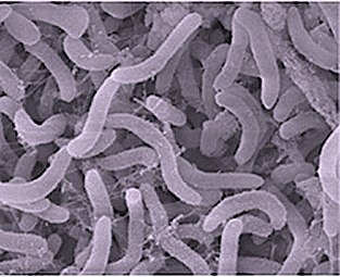  Pelagibacter ubique, the most abundant bacteria in the ocean, plays a major role in the global carbon cycle

Export processes in the ocean with connections to the ocean's biological pump and the pelagic food web. Light blue waters represent the euphotic zone while darker blue waters represent the twilight zone. Shown also is the how these these components are sampled and remotely sensed from ships, satellites, and autonomous vehicles.

Role of the microbial community in the marine carbon cycle

Marine export production

Marine methane paradox

• New Study Explains Mysterious Source of Greenhouse Gas Methane in the Ocean Woods Hole Oceanographic Institution, 21 November 2016.
• Repeta, Daniel J. et al.(2016) "Marine methane paradox explained by bacterial degradation of dissolved organic matter". Nature Geoscience. doi:10.1038/ngeo2837.

Polar webs

Part of an Arctic food web showing a network of food chains

Definitions:[11]

• A food web is a group of predators and prey that interact in a habitat or ecosystem
• A stressor is a factor that reduces the health or productivity of an ecosystem (i.e., causes stress)

Antarctic

Differences between the Arctic and the Antarctic regions
	Arctic	Antarctic
Geology	An ocean, partly frozen in the form of a massive ice cap. The Arctic ice cap floats on the surface of the Arctic Ocean, which plunges an average depth below of 1,000 metres.	A frozen continent covered almost entirely with glaciers. The Antarctic has ice mountains that rise to 4,900 metres, and is surrounded by the Southern Ocean.
Ocean currents and temperature	affected by warm waters of the gulf stream. A lot warmer than the Antarctic.	the ocean surrounding the Antarctic landmass is dominated by the Antarctic Circumpolar Current which allows little circulation of heat from other regions. This leads to extreme low temperatures (average -55 °C) and is the reason for the existing ice sheet.
Animal life	The arctic fox as well as marine mammals like polar bears, walrus, seals, and whales. Birds like puffins, fulmars, and other bird species.	Penguins and marine mammals like whales and seals
Human populations	Indigenous population (Inuits, Indians, Siberians) and enduring settlements	Historically deserted though today there are impermanent settlements for scientists.

Phytoplankton in the seasonal and marginal ice zones

Physical constraints on phytoplankton (A) before and (B) after climate change. Ovals represent the depth of mixing and arrow thickness reflect relative rates. Blue dashed line denotes the location of the pycnocline; and the red dashed line depicts the approximated depth for 1% surface irradiance.

SST: sea surface temperature

"Phaeocystis pouchetii... is one of the few non-diatom algae which is exceedingly plentiful in southern Antarctic waters. Phaeocystis occurs in either a unicellular motile form or a colonial palmelloid stage which can be large enough to be visible to the naked eye. This alga is very widely distributed in warm and temperate waters as well as in Antarctic and Arctic seas. Its gelatinous blooms are sometimes known as "Dutchman's baccy juice", and the jelly-like colonies are so thick that they clog plankton nets. Extensive blooms of Phaeocystis have been reported in the Ross Sea (El-Sayed et al., 1983) where high cell concentrations extended from the surface to depths of 100–150 m. Distinct discoloration of the water (greenish-grey to greenish-brown) accompanied this bloom, resulting in considerable submarine light attenuation."

• FOR IMAGE --> Bender, S.J., Moran, D.M., McIlvin, M.R., Zheng, H., McCrow, J.P., Badger, J., DiTullio, G.R., Allen, A.E. and Saito, M.A. (2018) "Colony formation in Phaeocystis antarctica: connecting molecular mechanisms with iron biogeochemistry". Biogeosciences, 15(16). doi:10.5194/bg-15-4923-2018. full text
• The marine environment - Discovering Antarctica <======= E X P L O R E
• Antarctica Food Chains and Food Webs

Anthropogenic effects

From Limacina helicina... Pteropods are strict pelagic mollusks that are highly adapted to life in the open ocean. They are actively swimming in the water. Limacina helicina is a holoplanktonic species. Habitat of Limacina helicina is upper epipelagic and glacial. It lives in temperatures from -0.4 °C to +4.0 °C or rarely up to 7 °C. Limacina helicina of the size from 0.2 to 0.4 mm lives mainly in depths from 0 m to 50 m. Larger pteropods lives from 0 m to 150 m. Already Constantine John Phipps mentioned its "innumerable quantities" in arctic seas in 1774. Limacina helicina is a major component of the polar zooplankton. It can comprise more than 50% of total zooplankton abundance (number of individuals per unit volume). Species of the clade Thecosomata produce a fragile external calcium carbonate shell, which could serve as a [[Sailing The aragonitic composition of the shell makes it very sensitive to dissolution. Aragonite is a metastable form of calcium carbonate and it is more soluble in seawater than calcite. Because of its highly soluble aragonite shell and polar distribution, Limacina helicina may be one of the first organisms affected by ocean acidification, and it is therefore a key indicator species of this process. A decline of pteropod populations would likely cause dramatic changes to various pelagic ecosystems. Shelled pteropods also play a geochemical role in carbon cycle in the oceans, as they contribute to the export of calcium carbonate and can represent a major component of the carbon transport to the deep ocean. Researchers found 24-53% individuals of Limacina helicina with shells damaged by dissolution off the U.S. West Coast in 2011.

See also

• Remineralisation

External links

• Ocean Color Time Series NASA
• Upwelling (Italian wikipedia)

Mixotrophic plankton

Mixotrophic plankton that combine phototrophy and heterotrophy – table based on Stoecker et. al., 2017
General types	Description		Example		Further examples
Bacterioplankton	Photoheterotrophic bacterioplankton			Vibrio cholerae	Roseobacter spp. Erythrobacter spp. Gammaproteobacterial clade OM60 Widespread among bacteria and archaea
Phytoplankton	Called constitutive mixotrophs by Mitra et. al., 2016. Phytoplankton that eat: photosynthetic protists with inherited plastids and the capacity to ingest prey.			Ochromonas species	Ochromonas spp. Prymnesium parvum Dinoflagellate examples: Fragilidium subglobosum,Heterocapsa triquetra,Karlodinium veneficum,Neoceratium furca,Prorocentrum minimum
Zooplankton	Called nonconstitutive mixotrophs by Mitra et. al., 2016. Zooplankton that are photosynthetic: microzooplankton or metazoan zooplankton that acquire phototrophy through chloroplast retentiona or maintenance of algal endosymbionts.
	Generalists	Protists that retain chloroplasts and rarely other organelles from many algal taxa			Most oligotrich ciliates that retain plastidsa
	Specialists	1. Protists that retain chloroplasts and sometimes other organelles from one algal species or very closely related algal species		Dinophysis acuminata	Dinophysis spp. Myrionecta rubra
		2. Protists or zooplankton with algal endosymbionts of only one algal species or very closely related algal species		Noctiluca scintillans	Metazooplankton with algal endosymbionts Most mixotrophic Rhizaria (Acantharea, Polycystinea, and Foraminifera) Green Noctiluca scintillans
aChloroplast (or plastid) retention = sequestration = enslavement. Some plastid-retaining species also retain other organelles and prey cytoplasm.

Locomotion of protists

A bacterial flagellum rotated by a molecular motor at its base

Paramecium feeding on bacteria

Protists are often categorised according to their mode of locomotion. Most unicellular protists are motile and can generate movement using flagella, cilia or pseudopods. Cells which use flagella are usually referred to as flagellates, cells which use cilia for movement are usually referred to as ciliates, and cells which use pseudopods are usually referred to as amoeba or amoeboids.

Flagellates include bacteria as well as protists. The rotary motor model used by bacteria uses the protons of an electrochemical gradient in order to move their flagella. Torque in the flagella of bacteria is created by particles that conduct protons around the base of the flagellum. The direction of rotation of the flagella in bacteria comes from the occupancy of the proton channels along the perimeter of the flagellar motor.

Ciliates use small flagella called cilia to power their movement through the water. One ciliate will generally have hundreds to thousands of cilia that are densely packed together in arrays. During movement, an individual cilium deforms using a high-friction power stroke followed by a low-friction recovery stroke. Since there are multiple cilia packed together on an individual organism, they display collective behavior in a metachronal rhythm. This means the deformation of one cilium is in phase with the deformation of its neighbor, causing deformation waves that propagate along the surface of the organism. These propagating waves of cilia are what allow the organism to use the cilia in a coordinated manner to move. A typical example of a ciliated microorganism is the Paramecium, a one-celled, ciliated protozoan covered by thousands of cilia. The cilia beating together allow the Paramecium to propel through the water at speeds of 500 micrometers per second.

Protists according to how they move
Type of protist	Movement mechanism	Description	Example		Other examples
Flagellate	flagella	use one or several flagella. A flagella is a lash-like appendage that protrudes from the cell body of some protists (as well as some bacteria).		Cryptophytes	Excavates are considered to be the most basal flagellate lineage. Other flagellates include dinoflagellates, choanoflagellates, most green algae, some radiolarians (probably gametes), foraminiferans (as gametes)
Ciliate	cilia	use multiple cilia, which are small flagella, to power themselves through the water		Paramecium bursaria - click to expand and see cillia	Foraminiferans, and some marine amoebae, ciliates and flagellates.
Amoeba (Amoeboids)	pseudopods	Amoeba have the ability to alter shape by extending and retracting pseudopods.		Amoeba proteus	are found in every major lineage of protists. Amoeboid cells occur not only among the protozoa, but also in fungi, algae, and animals.

Haeckel, Turing and radiolarian morphology

Forminarians

          Drawings by Haeckel 1904 (click for details)

Diatoms

          Drawings by Haeckel 1904 (click for details)

Radiolarians

          Drawings by Haeckel 1904 (click for details)

Turing and radiolarian morphology

Radiolarians come in many shapes

Shell micrographs

      Computer simulations of Turing patterns on a sphere
        closely replicate some radiolarian shell patterns      

Radiolarians are unicellular protists with elaborate silica shells

Silicate shell made by a radiolarian which once lived inside

Spumellaria: Hexastylus sp.

Spumellaria: Stylosphaeridae sp.

• Kunstformen der Natur (Art Forms in Nature)
• The Chemical Basis of Morphogenesis

Turing, A.M. (1990) "The chemical basis of morphogenesis". Bulletin of mathematical biology, 52(1-2): 153–197. SEE: http://www.dna.caltech.edu/courses/cs191/paperscs191/turing.pdf

• Turing patterns on a sphere, 1999...

"Turing systems were originally put forward to explain the chemical basis of morphogenesis, that is, how a zygote, which is a spherical object, can acquire a form with a smaller symmetry. Our calculations are ideal to revive this discussion. Very simple unicellular organisms present complicated symmetry breaking that should be compared with Turing’s predictions. Among the simplest ones are the Radiolaria. These micro-organisms present very beautiful patterns of silicates formed on their membranes. There is an incredible variety of forms, some are spherical and others are conical or elongated. Many, although not all, of the radiolaria skeletons have hexagonal structuring on their surfaces. In Fig. 7 we show photographs of two selected common spherical radiolaria. Notice the resemblance of the skeleton in Fig. 7!a" with our pattern in Fig. 5, and the remarkable correspondence of the skeleton in Fig. 7!b" with our pattern in Fig. 6"...

". The skeleton of microscopic sea animals, called Radiolaria, have spherical form with motifs arranged in tetrahedral, octahedral, icosahedral, and other more complex symmetries #6$. Notably, the skeleton of a Radiolarian called Aulonia hexagona shows a fairly distorted triangular lattice spread out over the sphere !see Fig. 55 in Ref. #11$". This pattern contains also distorted pentagons as in the example we give in Fig. 6."

https://www.researchgate.net/profile/Rafael_Barrio/publication/11398635_Turing_patterns_on_a_sphere/links/004635334571f485c0000000.pdf

Numerical analyses have already been performed by Varea et al. [11], and their results compare favorably with the structures of various radiolaria.

computer matches were very good

Pattern formation on a sphere

skeletal patterns in radiolaria allows us to compare theoretical results with spherical biological systems such as the skeletons of several radiolaria

Their simulations show the emergence of different symmetries on this surface and are reminiscent of skeletal patterns in radiolaria

Radiolarian patterns can arise naturally from a uniform sphere

FROM: Patterns in nature... Ernst Haeckel (1834–1919) painted beautiful illustrations of marine organisms, in particular Radiolaria, emphasising their symmetry to support his faux-Darwinian theories of evolution.... In 1952, Alan Turing (1912–1954), better known for his work on computing and codebreaking, wrote The Chemical Basis of Morphogenesis, an analysis of the mechanisms that would be needed to create patterns in living organisms, in the process called morphogenesis. He predicted oscillating chemical reactions, in particular the Belousov–Zhabotinsky reaction. These activator-inhibitor mechanisms can, Turing suggested, generate patterns (dubbed "Turing patterns") of stripes and spots in animals, and contribute to the spiral patterns seen in plant phyllotaxis.

a seminal paper... which was subsequently shown to predict the type of patterns found in radiolarians, such as in the photo below.

• Bernard Richards
• pioneering work on morphogenesis
• The Turing Guide -

Turing’s theory of morphogenesis

• Turing pattern
• The Turing Guide

FROM: https://www.sciencedaily.com/releases/2016/08/160809095259.htm "Geologists appreciate the radiolarian ooze very much, because the alien-looking creatures have lived on our planets for approximately 500 million years. Therefore, fossil radiolarians are very useful for dating geological structures... "Ernst Haeckel and other former natural scientists classified the radiolarians according to their morphology, that is their appearance in a broad sense. But it is not always true that organisms are genetically related even if they have a similar appearance," Krabberød explains... Already around 1870, Ernst Haeckel discovered a photosynthesizing algae living in colonies together with radiolarians, in a common gel secreted by the radiolarian hosts. Organisms living together like this are called symbionts. Anders Krabberød has, by using DNA analysing techniques, shown that several marine species in the protistan alveolate group(link is external) also seem to be living as symbionts with radiolarians, but these are hiding themselves inside the siliceous exoskeletons of certain species... Radiolarians are exclusive salt water species and can be found in every ocean on Earth. Some of them have pseudopodia -- "false feet" -- that can be used for different purposes."

FROM: https://blogs.scientificamerican.com/artful-amoeba/proteus-how-radiolarians-saved-ernst-haeckel/ "Radiolarians are tiny protists that live inside intricate silica shells. Because silica is impervious to the acids that often dissolve shells made of calcium carbonate at great depth, they make up a huge proportion of the sludge found on deep sea beds. They extend tiny pseudopods out from their shell to capture food, and sometimes they house algae to help feed them... They were among the earliest eukaryotes to evolve at the end of the Pre-Cambrian, 550 million years ago, and their shells have varied so much over time that they are useful for dating petroleum beds and geological formations. But why do they have those shells, and what force could be selecting for the endless variety in their structure? I do not know... "

FROM: https://www.sciencedirect.com/topics/earth-and-planetary-sciences/radiolaria "Radiolaria are single-celled marine planktonic protozoa that secrete an opal skeleton composed of a number of architectural elements (radial spicules, internal bars, external spines) that are joined together to form regular symmetrical structures. The skeletons are usually smaller than 2 mm and commonly between 100 and 250 μm in diameter. Radiolaria can be solitary and colonial, the latter producing centimetre- to metre-sized aggregates (Flügel, 2004). Radiolaria are found exclusively in marine sediments, proving some information about the nature of soil parent materials (Clarke, 2003; Stoops, 2003)."

translucent cage over 500 million years old, amongst the earliest skeletonized life forms

Calcite and silicate

From calcium carbonate...

"In warm, clear tropical waters corals are more abundant than towards the poles where the waters are cold. Calcium carbonate contributors, including plankton (such as coccoliths and planktic foraminifera), coralline algae, sponges, brachiopods, echinoderms, bryozoa and mollusks, are typically found in shallow water environments where sunlight and filterable food are more abundant. Cold-water carbonates do exist at higher latitudes but have a very slow growth rate. The calcification processes are changed by ocean acidification... Where the oceanic crust is subducted under a continental plate sediments will be carried down to warmer zones in the asthenosphere and lithosphere. Under these conditions calcium carbonate decomposes to produce carbon dioxide which, along with other gases, give rise to explosive volcanic eruptions... The carbonate compensation depth (CCD) is the point in the ocean where the rate of precipitation of calcium carbonate is balanced by the rate of dissolution due to the conditions present. Deep in the ocean, the temperature drops and pressure increases. Calcium carbonate is unusual in that its solubility increases with decreasing temperature. Increasing pressure also increases the solubility of calcium carbonate. The carbonate compensation depth can range from 4,000 to 6,000 meters below sea level."

"Sediment cores from the ocean floor contain types of information that scientists use to better understand the fluctuations of global climate. Perhaps the most important information is that gleaned from the microscopic shells of animals such as this, called planktonic Foraminifera ("forams" for short). Forams provide two main types of information. First of all, different species of forams prefer different ocean temperature and nutrient conditions. . Scientists can therefore learn much about the climatic conditions of a core site in the past by looking at which species once inhabited the area. Secondly, the shells of forams effectively lock in the oxygen and carbon isotopic composition of the waters in which they formed. Because past periods of glaciation changed the relative quantities of heavy oxygen (18O) and light oxygen (16O), scientists can use the isotopic composition of foram shells as a proxy signal for past changes in global ice volume. Other chemical measures are available as well by studying the composition of the shells. Data from ocean cores about past glaciation matches Milankovitch's theory remarkably well."

• Biomineralization
• Carbonate–silicate cycle

In many parts of the world, silica is the major constituent of sand.

From silicon dioxide...

"For well over a billion years, silicification in and by cells has been common in the biological world. In the modern world it occurs in bacteria, single-celled organisms, plants, and animals (invertebrates and vertebrates). Prominent examples include:

• Tests or frustules (i.e. shells) of diatoms, Radiolaria and testate amoebae.
• Silica phytoliths in the cells of many plants, including Equisetaceae, practically all grasses, and a wide range of dicotyledons.
• The spicules forming the skeleton of many sponges."

From: Biomineralization

Some calcareous sponges (Ernst Haeckel, Kunstformen der Natur).

"Biomineralization is the process by which living organisms produce minerals, often to harden or stiffen existing tissues. Such tissues are called mineralized tissues. It is an extremely widespread phenomenon; all six taxonomic kingdoms contain members that are able to form minerals, and over 60 different minerals have been identified in organisms. Examples include silicates in algae and diatoms, carbonates in invertebrates, and calcium phosphates and carbonates in vertebrates. These minerals often form structural features such as sea shells and the bone in mammals and birds. Organisms have been producing mineralised skeletons for the past 550 million years. Ca carbonates and Ca phosphates are usually crystalline, but silica organisms (sponges, diatoms...) are always non crystalline minerals. Other examples include copper, iron and gold deposits involving bacteria. Biologically-formed minerals often have special uses such as magnetic sensors in magnetotactic bacteria (Fe₃O₄), gravity sensing devices (CaCO₃, CaSO₄, BaSO₄) and iron storage and mobilization (Fe₂O₃•H₂O in the protein ferritin).

IUPAC definition

Biomineralization: Complete conversion of organic substances to inorganic derivatives by living organisms, especially micro-organisms.

The first evidence of biomineralization dates to some 750 million years ago, and sponge-grade organisms may have formed calcite skeletons 630 million years ago. But in most lineages, biomineralization first occurred in the Cambrian or Ordovician periods. Organisms used whichever form of calcium carbonate was more stable in the water column at the point in time when they became biomineralized, and stuck with that form for the remainder of their biological history (but see for a more detailed analysis). The stability is dependent on the Ca/Mg ratio of seawater, which is thought to be controlled primarily by the rate of sea floor spreading, although atmospheric CO₂ levels may also play a role."

Type of mineralization	Examples of organisms
Calcium carbonate (calcite or aragonite)	foraminifera coccolithophores calcareous sponge spicules corals Archaeocyatha bryozoans brachiopod and mollusc shells Echinoderms Serpulidae
Silica	radiolarians diatoms most sponge spicules
Apatite (phosphate carbonate)	enamel (Vertebrate teeth) Vertebrate bone conodonts

Images

Selections from Ernst Haeckel's 1904 Kunstformen der Natur (Art Forms of Nature), showing pennate (left) and centric (right) frustules

sponge spicule

Planktonic protists: plants and grazers

Star stick diatom (NOAA)

Wagon wheel diatom (NOAA)

See also: Calcareous ooze, Calcium cycle, Biogenic silica, Sedimentary rock, Biomineralization, Seabed § Sediments, and Sediment–water interface

from coccolithophore, terrigenous sediment and pelagic sediment...

"Where biogenic constituents compose less than 30 percent of the total, the deposit is called a deep-sea clay, brown mud, or red clay".

The skeletons are elaborate external hard mineral shells, usually made of silica (as in radiolaria and diatoms) or of calcium carbonate (as in foraminifera and coccoliths).

• biogenic silica

radiolarians

Radiolarians are unicellular with diameters from 0.1 to 0.2 mm, and grow intricate mineral skeletons. They are found as zooplankton throughout the ocean, and their skeletal remains make up much of the cover of the ocean floor as siliceous ooze. Due to their rapid species turn-over, they are important diagnostic microfossils found from the Cambrian onwards.

diatoms

foraminiferans

FROM: https://ucmp.berkeley.edu/foram/foramintro.html "Foraminifera (forams for short) are single-celled protists with shells. Their shells are also referred to as tests because in some forms the protoplasm covers the exterior of the shell. ... Radiating from the opening are fine hairlike reticulopodia, which the foram uses to find and capture food... A single individual may have one or many nuclei within its cell. The largest living species have a symbiotic relationship with algae, which they "farm" inside their shells. Other species eat foods ranging from dissolved organic molecules, bacteria, diatoms and other single celled phytoplankton, to small animals such as copepods. They move and catch their food with a network of thin extensions of the cytoplasm called reticulopodia, similar to the pseudopodia of an amoeba, although much more numerous and thinner."

FROM: https://www.ncbi.nlm.nih.gov/pubmed/14601411 "Foraminiferal research lies at the border between geology and biology. Benthic foraminifera are a major component of marine communities, highly sensitive to environmental influences, and the most abundant benthic organisms preserved in the deep-sea fossil record. These characteristics make them important tools for reconstructing ancient oceans."

Most foraminiferans have calcareous tests, composed of calcium carbonate. A few forams have tests made of organic material, and in one genus of silica. Tests as fossils are known from as far back as the Cambrian period, and many marine sediments are composed primarily of them. For instance, the limestone that makes up the pyramids of Egypt is composed almost entirely of nummulitic benthic Foraminifera. It is estimated reef Foraminifera generate about 43 million tons of calcium carbonate per year.

foraminifera FROM: https://www.youtube.com/watch?v=JLSa8cGJixQ foraminifera go back about 650 years ago The typical foraminifera is about the size of a period at the end of a sentence... foraminifera reflect environmental change - they are very sensitive indicators of environmental change. One way foraminifera can tell us something is by chemical analysis of the shells. You can look at the isotopic composition of the oxygen and the carbon and trace element concentrations in the shell. That means we can say things about direct temperature of the past. It can tell us about the polar ice caps. It can tell something about how much photosynthesis was going on in the surface of the ocean, and that can tell us something about the CO2 levels in the atmosphere.

See Paleocene–Eocene Thermal Maximum for data derives from foraminifera fossils

foraminifera are big players in constructing what we know about palaeoclimatology.

Genetic studies have identified the naked amoeba Reticulomyxa and the peculiar xenophyophores as foraminiferans without tests.

Most foraminifera species are benthic, though 40 morphospecies are planktonic.

Planktonic foraminifera are represented by many species with worldwide occurrence in broad latitudinal and temperature belts, floating in the surface or near-surface waters of the open ocean as part of the marine zooplankton. Benthic foraminifera are as successful as the planktonic foraminifera group and even more abundant in modern seas and can live attached or free, at all depths.

---

coccolithophores

Ooze is pelagic sediment that consists of at least 30% of microscopic remains of either calcareous or siliceous planktonic debris organisms. Oozes can be defined by and classified according to the predominate organism that compose them. For example, there are diatom, coccolith, foraminifera, globigerina, pteropod, and radiolarian oozes. Oozes are also classified and named according to their mineralogy, i.e. calcareous or siliceous oozes. Whatever their composition, all oozes accumulate extremely slowly, at no more than a few centimeters per millennium.

Calcareous ooze is ooze that is composed of at least 30% of the calcareous microscopic shells—also known as tests—of foraminifera, coccolithophores, and pteropods. This is the most common pelagic sediment by area, covering 48% of the world ocean's floor. This type of ooze accumulates on the ocean floor at depths above the carbonate compensation depth. It accumulates more rapidly than any other pelagic sediment type, with a rate that varies from 0.3–5 cm/1000 yr.

Siliceous ooze is ooze that is composed of at least 30% of the siliceous microscopic "shells" of plankton, such as diatoms and radiolaria. Siliceous oozes often contain lesser proportions of either sponge spicules, silicoflagellates or both. This type of ooze accumulates on the ocean floor at depths below the carbonate compensation depth. Its distribution is also limited to areas with high biological productivity, such as the polar oceans, and upwelling zones near the equator. The least common type of sediment, it covers only 15% of the ocean floor. It accumulates at a slower rate than calcareous ooze: 0.2–1 cm/1000 yr.

---

Diatoms are divided into two groups that are distinguished by the shape of the frustule: the centric diatoms and the pennate diatoms.

Pennate diatoms are bilaterally symmetric. Each one of their valves have openings that are slits along the raphes and their shells are typically elongated parallel to these raphes. They generate cell movement through cytoplasm that streams along the raphes, always moving along solid surfaces.

Centric diatoms are radially symmetric. They are composed of upper and lower valves - epitheca and hypotheca - each consisting of a valve and a girdle band that can easily slide underneath each other and expand to increase cell content over the diatoms progression. The cytoplasm of the centric diatom is located along the inner surface of the shell and provides a hollow lining around the large vacuole located in the center of the cell. This large, central vacuole is filled by a fluid known as "cell sap" which is similar to seawater but varies with specific ion content. The cytoplasmic layer is home to several organelles, like the chloroplasts and mitochondria. Before the centric diatom begins to expand, its nucleus is at the center of one of the valves and begins to move towards the center of the cytoplasmic layer before division is complete. Centric diatoms have a variety of shapes and sizes, depending on from which axis the shell extends, and if spines are present.

Misc

• 
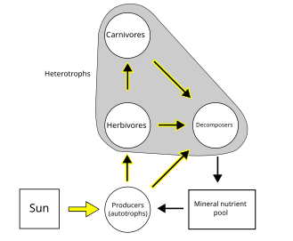  Simple Food Web
• 
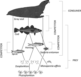  Central Baltic Food Web Model
• 
  build up of toxins in a food chain
• 
  Carbonate-Silicate Cycle (Carbon Cycle focus)
• 
  Carbon-Slicate Cycle Feedbacks
• 
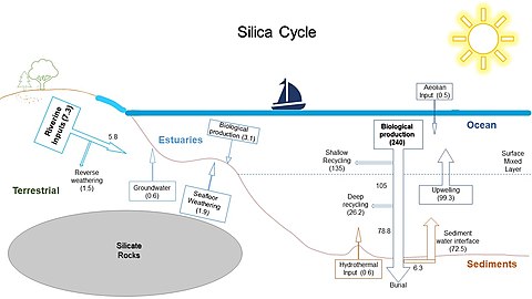  Silica cycle draft
• 
  Marine Silica Cycle
• 
  Bluebell tunicates

Algae

• 
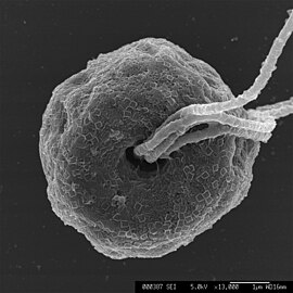  Flagellar pit of Pyramimonas sp.
• 
  Flagellar pit of Pyramimonas sp.
• 
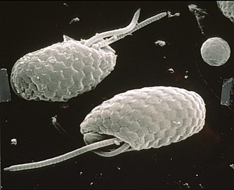  Two Cryptophytes
• 
  Cryptophytes under light microscope
• 
  Euglena viridis
• 
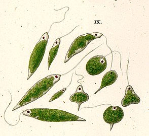
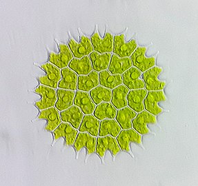  Colony of Pediastrum algae (freshwater)
• 
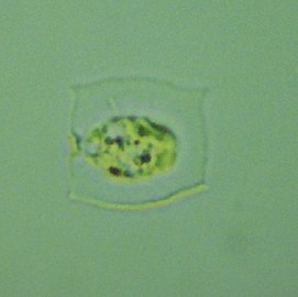  green algae Pteromonas
• 
  Green algae, Chlorophyceae - chlorophytes
• 
  Colony of green alga, Pediastrum (light micrograph) (freshwater)
• 
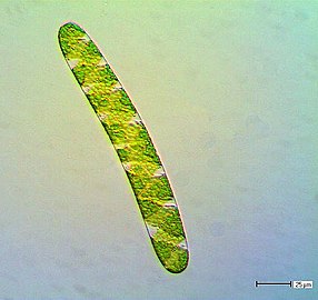  Spirotaenia, a genus of basal green algae that may be sister to the Chlorokybophyceae
• 
  Haeckel Siphoneae
• 
  Green algae on coastal rocks
• 
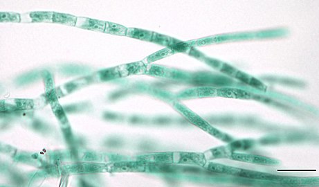  Photomicrograph of multiple strands of Stigeoclonium
• 
  Coelastrum sp.
• 
  Green algae?
• 
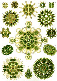  Haeckel Melethallia
• 
  largest marine genera
• 
• 
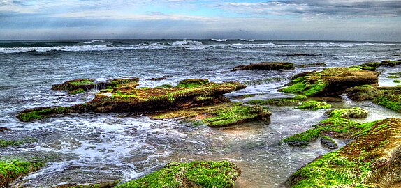
  Acetabularia acetabulum
• 
• 
• 
• 
• 
• 
• 
  Braarudosphaera bigelowii
• 
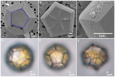
  Brown algae
• 
  kelp beds
• 
• 
• 
  Red algae, Cyanidium sp.

Penard Collection

• 
  Amoeba from the Amoeba Collection made by Eugène Penard at the beginning of the 20th century
• 
  Amoeba proteus

Pamphagus granulatus

• 
  A Rhizaria covered in diatoms, from Eugène Penard's Amoeba Collection made by at the beginning of the 20th century
• 
• 
• 
• 
• 
• 
• 

misc protozoa

• 
  cytostome (mouth), cytoproct (anus), contractile vacuole, ectoplasm, endoplasm,
• 
  Stramenopile (heterokont) have two, unequal flagella
• 
  Fucus receptacle with sterile paraphysesz, oogonium, and an ostiole where the opening in the surface of the receptacle is
• 
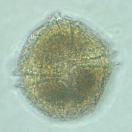  Lingulodinium polyedrum, a species of photosynthetic dinoflagellates that can cause red tides and bioluminescent displays on beaches
• 
  Electron microscope image of Chlamydomonas reinhardtii, a single-cell green alga about that swims with two flagella - used as a model organism for research on fundamental questions in cell and molecular biology
• 
  Sea lettuces are edible green algae common along the coasts
• 
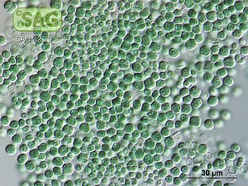  Chroococcidiopsis is one of the most primitive cyanobacteria known. It can photsynthesize in far-red light, and might be suitable for future colonising Mars.
• 
  Klebsormidium bilatum are charophyte green alga forming multicellular, non-branching filaments
• 
• 
• 
• 
• 
• 
• 
• 
• 
• 
• 

Choanoflagellate

Choanoflagellates - a group of free-living unicellular and colonial flagellate eukaryotes considered to be the closest living relatives of the animals.

• 
• 
• 
• 
• 
• 
• 
• 
• 
• 
• 
• 
• 
• 
• 
• 

Marine diatoms

• 
  Inner and external plates of a single valve of the centric diatom Coscinodiscus wailesii
• 
• 
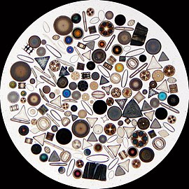
  diatoms
• 
• 
• 
  diatom
• 
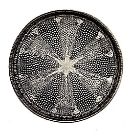  Diatom, Helipelta metil
• 
  Diatom, Triceratium favus
• 
  diatoms
• 
  diatoms
• 
  diatoms
• 
  diatom
• 
• 
• 
• 
• 
• 
• 
• 
• 
• 
• 
• 
• 
  diatom
• 
• 
• 
  Navicula oblonga
• 
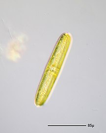
  Centric diatom
• 
  diatoms
• 
  diatoms
• 
  centric diatom
• 
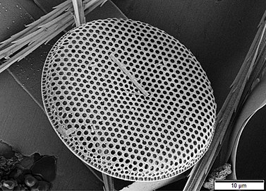  diatoms
• 
  pennate diatom
• 
  pennate diatom
• 
  pennate diatom
• 
  various diatoms
• 
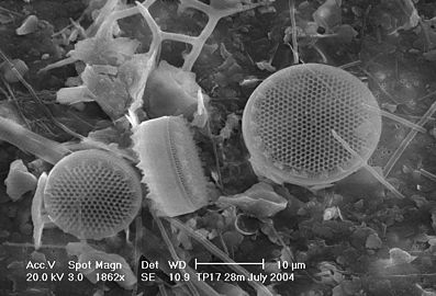  diatoms
• 
  diatoms
• 
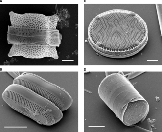  diatoms ##
• 
  diatoms
• 
  diatoms
• 
  diatoms
• 
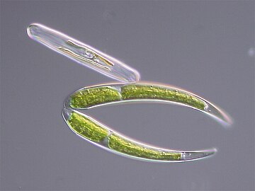  Closterium sp. (with unknown diatom), mitotic phase
• 
  Biddulphia pulchella
• 
  Biddulphia sp.
• 
  The diatom Phaeodactylum tricornutum can grow in the absence of silicon, and can survive without making silicified frustules.
• 
  Diatom
• 
  The pennate diatom Fragilariopsis kerguelensis is the most abundant diatom in the Antarctic Seas".
• 
  Diatom Isthmia nervosa
• 
  Haeckel Diatomea
• 
  Haeckel Diatomea
• 
  Diatom Odontella aurita
• 
  Surirella spiralis
• 
• 
  Pleurosigma angulatum diatoms
• 
  Diatom frustle
• 
  Диатомит Инзенского месторождения, электронный микроскоп
• 
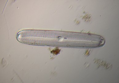  Diatom
• 
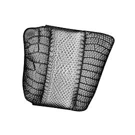  Diatom - Isthmia nervosa
• 
  Diatom - Champylodiscus sp
• 
• 
• 

Radiolarians

• 
• 
• 
  Radiolarian protists drawn by Haeckel 1904
• 
  Radiolarians (Haeckel)
• 
  Radiolarian
• 
  Fossil radiolarian
• 
• 
• 
• 
• 
• 
• 
• 
  Challenger
• 
  Haeckel Radiolaria: Spumellaria
• 
  Haeckel Cyrtoidea
• 
  Haeckel Phaeodaria
• 
  Haeckel Acanthometra
• 
  Stylosphaera flexuosa
• 
  Radiolaria - Sijthoff
• 
  Haeckel - Discoidea
• 
• 
• 
• 
• 
  Haeckel Phaeodaria
• 
• 
• 
  Radiolarians
• 
• 
• 

Unidentified radiolarians

• 
  (not identified)
• 
  Halicalyptra petalospyris ?

Coccolithophores

• 
• 
• 
• 
• 
• 
• 
• 
• 
• 
• 
• 
• 
• 
• 
• 

Foraminiferans

• 
  Foraminiferan
• 
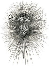  Test of a planktic foraminiferan with defensive spines
• 
  Test of Globigerina bulloides, an ooze-forming protozoan foraminiferan that is found as marine plankton
• 
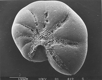  Benthic foram, Elphidium incertum
• 
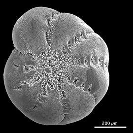  Benthic foram, Elphidium excavatum clavatum
• 
  Haeckel Thalamophora
• 
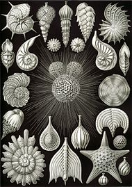  Haeckel Thalamophora
• 
  Haeckel Thalamophora
• 
  Planktonic foram
• 
• 
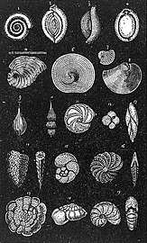  Calcareous Foraminifera
• 
  Elphidium, benthic foraminifera, about 400 µm ø
• 
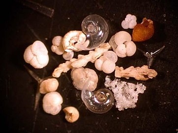  Planktonic foraminifera
• 
  Foraminifera
• 
  Foraminifera
• 
  Foraminifera
• 
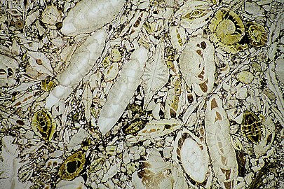  Foraminifera
• 
  Orbitolina texana foraminifera fossils
• 
  fossil foraminifera
• 
  Calcarina
• 
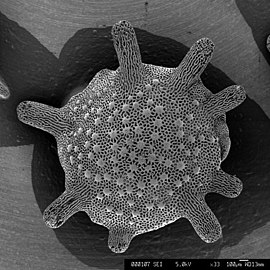
  Textilaria, a genus of benthic foraminifera
• 
  Live Ammonia tepida streaming granular ectoplasm for catching food etc
• 
  Dentalina commonis, which belongs to an order Lagenide of benthic foraminifera that have a finely perforated radial calcitic shell , in which the crystals appear wrapped by organic membranes.
• 
  section of Rotalia beccarii
• 
  Operculina section
• 
  Nummulitis lenticularis

Dinoflagellates

• 
• 
  Karenia brevis
• 
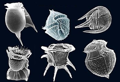  Dinoflagellates
• 
  The free-living unarmored dinoflagellata
• 
  The free-living unarmored dinoflagellata
• 
  The free-living unarmored dinoflagellata
• 
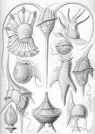  Haeckel Peridinea
• 
• 
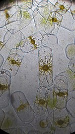  Colonial dinoflagellates
• 
• 
• 
  dinoflagellate cyst
• 
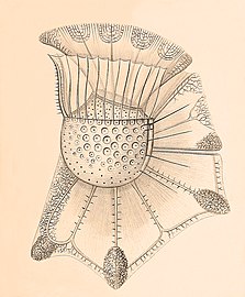  Planktonic dinoflagellate, Ornithocercus magnificus
• 
  Ornithocercus is a thecate dinoflagellate. This means they are armoured with overlapping cellulose plates collectively called a theca. Species range in length from 40-170 µm. They are therefore classed as microplankton
• 
• 
• 
• 
• 
• 
• 
• 
• 
• 
• 
• 
• 
• 
• 
• 
• 
• 
• 
• 
  Many dinoflagellates are encased in cellulose armor and have two flagella that fit in grooves between the plates. Movement of these two perpendicular flagella causes a spinning motion.
• 
• 
• 
• 
• 

Ciliates and amoeba

• 
  Ciliate Ciliophora
• 
  Suctoria sucking another ciliate
• 
  Ciliate Ciliophora
• 
• 
• 
• 
• 
• 
• 
  Hypotricher
• 
• 
• 
• 
• 
• 
• 
• 
• 
• 
• 
• 
• 
• 
  Tintinnid Tintinnopsis campanula
• 
• 
  Euplotes with amoeba
• 
• 
• 
• 
• 
• 
• 
• 
• 
• 
• 
• 
• 

Euglena

• 
• 
  Drawing of a Euglena single cell flagellate (fresh and saltwater)
• 

Gastrotricha

• 
  Gastrotricha
• 
  Gastrotricha
• 
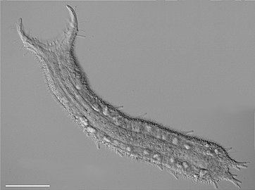  Gastrotricha

Fungi

• 
  Haeckel - Mycetozoa (slime moulds)

Gastropods

• 
  Undescribed species of deepwater nudibranch
• 
  Glaucus atlanticus

Miscellaneous

• 
  Bathyphysa conifera, sometimes called the "flying spaghetti monster", a bathypelagic species of siphonophore
• 
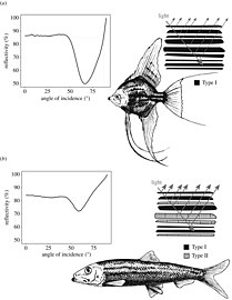  Reflectivity from silvery fish
• 
• 
  Microfossils
• 
  Protozoa
• 
  Planktonic jellyfish Medusae drift in the water column and move by contracting the muscles within the bell-like structure creating pulse-like movements. The tentacles contain harpoon-like stinging cells to capture small planktonic shrimp and crabs.
• 
  Paramecium
• 
  Paramecium caudatum and Stylonychia mytilus
• 
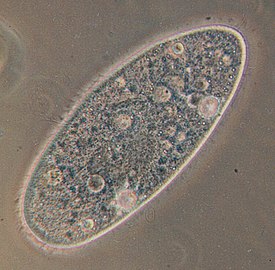
  Ctenophore
• 
  Radiata diversity
• 
  Terebellides horikoshii worm
• 
  Hydra (freshwater only)
• 
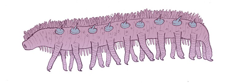  Onychodictyon, extinct lobopodan
• 
  Diagram of a typical animal cell. Organelles are labelled as follows: (1) Nucleolus; (2) Nucleus; (3) Ribosome; (4) Vesicle; (5) Rough endoplasmic reticulum; (6) Golgi apparatus; (7) Microtubule; (8) Smooth endoplasmic reticulum; (9) Mitochondrion; (10) Vacuole; (11) Cytoplasm; (12) Lysosome; (13) Centrioles
• 
• 
• 
• 
• 
• 
• 
• 
• 
• 
• 
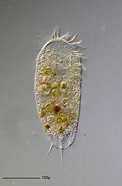
  Marine siphonophore
• 
  phytoplankton
• 
  Cyanobacteria Snowella
• 
  waterflea
• 
  Dinoflagellat (Neoceratium horridum) with diatom (Coscinodiscus radiatus)
• 
  Mnemiopsis leidyi