
William F. Egan
editWilliam F. Egan is well-known expert and author in the area of PLL's. The first and second editions of his book Phase-Lock Basics[1][2] as well as his books on Frequency Synthesis by Phase Lock[3][4] have been highly influential and remains a well-recognized reference among electrical engineers specializing in areas involving PLL's.
Egan's conjecture on the pull-in range of type II APLL
editIt is known that the hold-in and pull-in ranges for type II APLL for a given parameters are either infinite or empty. Moreover, for the second-order type II APLL if the the hold-in range is infinite then the pull-in range is also infinite (i.e. local stability implies global stability). W. Egan, вescribing the third-order type II APLL[3]: 176 ,[1]: 69, 168, 192 ,[2]: 59, 138, 161 , conjectured that it also has infinite pull-in range.
- ^ a b Egan, William F. (1998). Phase-Lock Basics (1st ed.). New York: John Wiley & Sons.
- ^ a b Egan, William F. (2007). Phase-Lock Basics (2nd ed.). New York: John Wiley & Sons.
- ^ a b Egan, William F. (1981). Frequency synthesis by phase lock (1st ed.). New York: John Wiley & Sons.
- ^ Egan, William F. (2011). Advanced Frequency Synthesis by Phase Lock (2nd ed.). New York: John Wiley & Sons.
Charge-pump phase-locked loop
edit
Charge-pump phase-locked loop (CP-PLL) is a modification of phase-locked loops with phase-frequency detector and square waveform signals. CP-PLL is design to quickly lock onto the phase of the incoming signal, achieving low steady state phase error[1].
Phase-frequency detector (PFD)
edit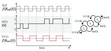
Phase-frequency detector (PFD) is triggered by the trailing edges of the reference (Ref) and controlled (VCO) signals. The output signal of PFD can have only three states: 0, , and . A trailing edge of the reference signal forces the PFD to switch to a higher state, unless it is already in the state . A trailing edge of the VCO signal forces the PFD to switch to a lower state, unless it is already in the state . If both trailing edges happen at the same time, then the PFD switches to zero.


Mathematical models of CP-PLL
editA first linear mathematical model of second-order CP-PLL was suggested by F. Gardner in 1980[1], a nonlinear model without the VCO overload was suggested by M. van Paemel in 1994 [2] and then refined by N. Kuznetsov et al. in 2019[3]. The closed form mathematical model of CP-PLL taking into account the VCO overload was derived in.
Continuous time model of the second order CP-PLL
editWithout loss of generality it is supposed that trailing edges of the VCO and Ref signals occur when the corresponding phase reaches an integer number. Let the time instance of the first trailing edge of the Ref signal is defined as . The PFD state is determined by the PFD initial state , the initial phase shifts of the VCO and Ref signals.


The relationship between the input current and the output voltage for a proportionally integrating (perfect PI) filter based on resistor and capacitor is as follows


where is a resistance, is a capacitance, and is a capacitor charge. The control signal adjusts the VCO frequency:


where is the VCO free-running (quiescent) frequency (i.e. for ), is the VCO gain (sensivity), and is the VCO phase. Thus the continuous time nonlinear mathematical model of CP-PLL is as follows


with the following discontinuous piece-wise constant nonlinearity

and the initial conditions . This model is a nonlinear, non-autonomous, discontinuous, switching system.

Discrete time model of the second-order Charge-pump PLL
edit
The reference signal frequency is assumed to be constant: where , and are a period, frequency and a phase of the reference signal. Let . Denote by the first instant of time such that the PFD output becomes zero (if , then ) and by the first trailing edge of the VCO or Ref. Further the corresponding increasing sequences and for are defined. Let . Then for the is a non-zero constant ( ). Denote by the PFD pulse width (length of the time interval, where the PFD output is a non-zero constant), multiplied by the sign of the PFD output: i.e. for and for . If the VCO trailing edge hits before the Ref trailing edge, then and in the opposite case we have , i.e. shows how one signal lags behind another. Zero output of PFD on the interval : for . The transformation[4] allows to reduce the number of parameters to two: Here is a normalized phase shift and is a ratio of the VCO frequency to the reference frequency . Finally, the discrete-time model of second order CP-PLL without the VCO overload[3][5]


where

This discrete-time model has the only one steady state at and allows to estimate the hold-in and pull-in ranges[5]

If the VCO is overloaded, i.e. is zero, or what is the same: or , then the additional cases of the CP-PLL dynamics have to be taken into account[6]. For any parameters the VCO overload may occur for sufficiently large frequency difference between the VCO and reference signals. In practice the VCO overload should be avoided.


Mathematical models of high-order CP-PLL
editNonlinear high-order mathematical models of CP-PLL models cannot be represented in closed form: the resulting transcendental equations can not be solved analytically without using approximations[7].
References
edit- ^ a b F. Gardner (1980). "Charge-pump phase-lock loops". IEEE Transactions on communications. 28 (11): 1849–1858.
- ^ M. van Paemel (1994). "Analysis of a charge-pump pll: A new model". IEEE Transactions on communications. 42 (7): 2490–2498.
- ^ a b N. Kuznetsov, M. Yuldashev, R. Yuldashev, M. Blagov, E. Kudryashova, O. Kuznetsova, and T. Mokaev (2019). "Comments on van Paemel's mathematical model of charge-pump phase-locked loop" (PDF). Differential Equations and Control Processes. 1: 109–120.
{{cite journal}}: CS1 maint: multiple names: authors list (link) - ^ P. Curran, C. Bi, and O. Feely (2013). "Analysis of a charge-pump PLL: A new model". International Journal of Circuit Theory and Applications. 41 (11): 1109–1135.
{{cite journal}}: CS1 maint: multiple names: authors list (link) - ^ a b N.V. Kuznetsov, A.S. Matveev, M.V. Yuldashev, R.V. Yuldashev (2020). "Nonlinear analysis of charge-pump phase-locked loop: the hold-in and pull-in ranges" (PDF). IFAC World Congress.
{{cite journal}}: CS1 maint: multiple names: authors list (link) - ^ N. Kuznetsov, M. Yuldashev, R. Yuldashev, M. Blagov, E. Kudryashova, O. Kuznetsova, T. Mokaev (2020). "Charge pump phase-locked loop with phase-frequency detector: closed form mathematical model". arXiv (1901.01468).
{{cite journal}}: CS1 maint: multiple names: authors list (link) - ^ C. Hedayat, A. Hachem, Y. Leduc, and G. Benbassat (1999). "Modeling and characterization of the 3rd order charge-pump PLL: a fully event-driven approach". Analog Integrated Circuits and Signal Processing (19(1)): 25–45.
{{cite journal}}: CS1 maint: multiple names: authors list (link)
Hidden attractor
editIn the bifurcation theory, a bounded oscillation that is born without loss of stability of stationary set is called a hidden oscillation. In the nonlinear control theory, the birth of hidden oscillation in time-invariant control system with bounded states means crossing the boundary of domain of parameters, where local stability of the stationary states implies global stability (see, e.g. Kalman's conjecture). If hidden oscillation (or a set of such hidden oscillations filling a compact subset of the phase space of dynamical system) attracts all nearby oscillations then it is called a hidden attractor. For dynamical system with unique equilibrium point, which is globally attractive, the birth of hidden attractor corresponds to the qualitative change in the behaviour from monostability to bi-stability. In general case, a dynamical system may turn out to be multistable and have coexisting local attractors in the phase space. While trivial attractors, i.e. stable equilibrium points, can be easily found analytically or numerically, the search of periodic and chaotic attractors can turn out to be a challenging problem (see, e.g. the second part of Hilbert's 16th problem).
Classification of attractors as being hidden or self-excited ones
editTo identify a local attractor in physical or numerical experiment, one needs to choose an initial system’s state in attractor’s basin of attraction and observe how system’s state, starting from this initial state, after a transient process visualizes the attractor. The classification of attractors as being hidden or self-excited reflect the difficulties of revealing basins of attraction and searching for the local attractors in the phase space.
Definition[1][2][3]. An attractor is called a hidden attractor if its basin of attraction does not intersect with a certain open neighbourhood of equilibrium points; otherwise it is called a self-excited attractor.
The classification of attractors as being hidden or self-excited was introduced by G. Leonov and N. Kuznetsov in connection with the discovery of the hidden Chua attractor [4][5][6][7] for the first time in 2009 year. Similarly, an arbitrary bounded oscillation, not necessarily having an open neighborhood as the basin of attraction in the phase space, is classified as a self-excited or hidden oscillation.
Self-excited attractors
editFor a self-excited attractor, its basin of attraction is connected with an unstable equilibrium and, therefore, the self-excited attractors can be found numerically by a standard computational procedure in which after a transient process, a trajectory, starting in a neighbourhood of an unstable equilibrium, is attracted to the state of oscillation and then traces it (see, e.g. self-oscillation process). Thus, self-excited attractors, even coexisting in the case of multistability, can be easily revealed and visualized numerically. In the Lorenz system, for classical parameters the attractor is self-excited with respect to all existing equilibria and can be visualized by any trajectory from their vicinities; however for some other parameters values there are two trivial attractors coexisting with a chaotic attractor which is a self-excited one with respect to the zero equilibrium only. Classical attractors in Van der Pol, Beluosov–Zhabotinsky, Rössler, Chua, Hénon dynamical systems are self-excited.
A conjecture is that the Lyapunov dimension of a self-excited attractor does not exceed the Lyapunov dimension of one of the unstable equilibria, the unstable manifold of which intersects with the basin of attraction and visualizes the attractor[8].
Hidden attractors
editHidden attractors have basins of attraction, which are not connected with equilibria and are “hidden” somewhere in the phase space. For example, the hidden attractors are attractors in the systems without equilibria: e.g. rotating electromechanical dynamical systems with Sommerfeld effect (1902), in the systems with only one equilibrium, which is stable: e.g. counterexamples to the Aizerman's conjecture (1949) and Kalman's conjecture (1957) on the monostability of nonlinear control systems. One of the first related theoretical problems is the second part of the second part of Hilbert's 16th problem on the number and mutual disposition of limit cycles in two-dimensional polynomial systems where the nested stable limit cycles are hidden periodic attractors. The notion of hidden attractor has become a catalyst for the discovery of hidden attractors in many applied dynamical models [1][9][10].
In general, the problem with hidden attractors is that there are no any general straightforward methods to trace or predict such states for the system’s dynamics (see, e.g. [11]). While for two-dimensional systems hidden oscillations can be investigated using analytical methods (see, e.g., the results on the second part of Hilbert's 16th problem), for the study of stability and oscillations in complex nonlinear multidimensional systems numerical methods are often used. In the multi-dimensional case the integration of trajectories with random initial data is unlikely to provide a localization of a hidden attractor since a basin of attraction may be very small and the attractor dimension itself may be much less than the dimension of the considered system. Therefore, for the numerical localization of hidden attractors in multi-dimensional space it is necessary to develop special analytical-numerical computational procedures [1][12][8], which allow one to choose initial data in the attraction domain of hidden oscillation (which does not contain neighborhoods of equilibria) and then to perform trajectory computation. There are corresponding effective methods based on homotopy and numerical continuation: a sequence of similar systems is constructed, such that for the first (starting) system the initial data for numerical computation of oscillating solution (starting oscillation) can be obtained analytically, and then the transformation of this starting oscillation in the transition from one system to another is followed numerically.
References
edit- ^ a b c Leonov G.A.; Kuznetsov N.V. (2013). "Hidden attractors in dynamical systems. From hidden oscillations in Hilbert-Kolmogorov, Aizerman, and Kalman problems to hidden chaotic attractor in Chua circuits". International Journal of Bifurcation and Chaos in Applied Sciences and Engineering. 23 (1): art. no. 1330002. doi:10.1142/S0218127413300024.
- ^ Bragin V.O.; Vagaitsev V.I.; Kuznetsov N.V.; Leonov G.A. (2011). "Algorithms for Finding Hidden Oscillations in Nonlinear Systems. The Aizerman and Kalman Conjectures and Chua's Circuits" (PDF). Journal of Computer and Systems Sciences International. 50 (5): 511–543. doi:10.1134/S106423071104006X.
- ^ Leonov, G.A.; Kuznetsov, N.V.; Mokaev, T.N. (2015). "Homoclinic orbits, and self-excited and hidden attractors in a Lorenz-like system describing convective fluid motion". European Physical Journal Special Topics. 224: 1421–1458. doi:10.1140/epjst/e2015-02470-3.
- ^ Kuznetsov N.V.; Leonov G.A.; Vagaitsev V.I. (2010). "Analytical-numerical method for attractor localization of generalized Chua's system". IFAC Proceedings Volumes. 43 (11): 29–33. doi:10.3182/20100826-3-TR-4016.00009.
- ^ Leonov G.A.; Vagaitsev V.I.; Kuznetsov N.V. (2011). "Localization of hidden Chua's attractors" (PDF). Physics Letters. 375 (23): 2230–2233. doi:10.1016/j.physleta.2011.04.037.
- ^ Leonov G.A.; Vagaitsev V.I.; Kuznetsov N.V. (2012). "Hidden attractor in smooth Chua systems" (PDF). Physica D. 241 (18): 1482–1486. doi:10.1016/j.physd.2012.05.016.
- ^ a b Kuznetsov, N.V.; Leonov, G.A.; Mokaev, T.N.; Prasad, A.; Shrimali, M.D. (2018). "Finite-time Lyapunov dimension and hidden attractor of the Rabinovich system". Nonlinear Dynamics. 92 (2): 267–285. doi:10.1007/s11071-018-4054-z.
- ^ Kuznetsov N. V.; Leonov G. A. (2014). "Hidden attractors in dynamical systems: systems with no equilibria, multistability and coexisting attractors". IFAC Proceedings Volumes (IFAC World Congress Proceedings). 47 (3): 5445–5454. doi:10.3182/20140824-6-ZA-1003.02501.
- ^ Kuznetsov, N.V.; Leonov, G.A.; Yuldashev, M.V.; Yuldashev, R.V. "Hidden attractors in dynamical models of phase-locked loop circuits: limitations of simulation in MATLAB and SPICE". Communications in Nonlinear Science and Numerical Simulation. 51: 39–49. doi:10.1016/j.cnsns.2017.03.010.
- ^ Chen, G.; Kuznetsov, N.V.; Leonov, G.A.; Mokaev, T.N. (2015). "Hidden attractors on one path: Glukhovsky-Dolzhansky, Lorenz, and Rabinovich systems". International Journal of Bifurcation and Chaos in Applied Sciences and Engineering. 27 (8): art. num. 1750115. doi:10.1142/S0218127417501152.