User:Hongshengzhao/sandbox

Lec 1: Connection with fluid dynamics, relativity, tide, potential

Stellar dynamics is the branch of astrophysics which describes in a statistical way the collective motions of stars subject to their mutual gravity. The essential difference from celestial mechanics is that the number of body $N\gg 10.$

Landau notations

Notation	Name	Description	Example	Limit definition
$f(n)=O(g(n))$	Big O;	$|f|$ is bounded above by g (up to constant factor) asymptotically	$\sin(n)=O(1)$	$\limsup _{n\to \infty }\left|{\frac {f(n)}{g(n)}}\right|<\infty$
$f(n)\sim g(n)$	On the order of	f is equal to g asymptotically	${\sin(n) \over n}\sim {1 \over n}$	$\lim _{n\to \infty }{\frac {f(n)}{g(n)}}=1$
$f(n)\approx g(n)$	Astronomically about	f is equal to g within a factor of $\pi$ or better]]	$\pi ^{2}\approx 10\approx e^{2}$	${\frac {1}{\pi }}\leq {\frac {f(n)}{g(n)}}\leq \pi$
$f(n)=o(g(n))$	Small Oh	f is dominated by g asymptotically	${\sin(n) \over n}=o(1)$	$\lim _{n\to \infty }{\frac {f(n)}{g(n)}}=0$

Typical galaxies have upwards of millions of macroscopic gravitating bodies and countless number of neutrinos and perhaps other dark microscopic bodies. Also each star contributes more or less equally to the total gravitational field, whereas in celestial mechanics the pull of a massive body dominates any satellite orbits.

Stellar dynamics also has connections to the field of plasma physics. The two fields underwent significant development during a similar time period in the early 20th century, and both borrow mathematical formalism originally developed in the field of fluid mechanics.

In accretion disks and stellar surfaces, the dense plasma or gas particles collide very frequently, and collisions result in equipartition and perhaps viscosity under magnetic field. We see various sizes for accretion disks and stellar atmosphere, both made of enormous number of microscopic particle mass, $(L/V,M/N)$

• $O(10^{-8}{\text{pc}}/500{\text{km/s}},1M_{\odot }/10^{55}=m_{p})$ at stellar surfaces,
• $O(10^{-4}{\text{pc}}/10{\text{km/s}},0.1M_{\odot }/10^{54}\sim m_{p})$ around Sun-like stars or km-sized stellar black holes,
• $O(10^{-1}{\text{pc}}/100{\text{km/s}},10M_{\odot }/10^{56}\sim m_{p})$ around million solar mass black holes (about AU-sized) in centres of galaxies.

The system crossing time scale is long in stellar dynamics, where it is handy to note that

$1000{\text{pc}}/1{\text{km/s}}=1000{\text{Myr}}={\text{HubbleTime}}/14.$

The long timescale means that, unlike gas particles in accretion disks, stars in galaxy disks very rarely see a collision in their stellar lifetime. However, galaxies collide occasionally in galaxy clusters, and stars have close encounters occasionally in star clusters.

As a rule of thumb, the typical scales concerned (see the Upper Portion of P.C.Budassi's Logarithmic Map of the Universe) are $(L/V,M/N)$

• $O(\mathrm {10pc/10km/s} ,1000M_{\odot }/1000)$ for M13 Star Cluster,
• $O(\mathrm {100kpc/100km/s} ,10^{11}M_{\odot }/10^{11})$ for M31 Disk Galaxy,
• $O(\mathrm {10Mpc/1000km/s} ,10^{14}M_{\odot }/10^{77}=m_{\nu })$ for neutrinos in the Bullet Clusters, which is a merging system of N = 1000 galaxies.

Key Concepts and Approximations of a gravitational potential field: grainy or smooth

Stellar dynamics involves determining the gravitational potential of a substantial number of stars. The stars can be modeled as point masses whose orbits are determined by the combined interactions with each other. Typically, these point masses represent stars in a variety of clusters or galaxies, such as a Galaxy cluster, or a Globular cluster. Without getting a system's gravitational potential by adding all of the point-mass potentials in the system at every second, stellar dynamicists develop potential models that can accurately model the system while remaining computationally inexpensive. The gravitational potential, $\Phi$, of a system is related to the acceleration and the gravitational field, $\mathbf {g}$ by:

$${\frac {d^{2}\mathbf {r_{i}} }{dt^{2}}}}=\mathbf {\vec {g}} =-\nabla _{\mathbf {r_{i}} }\Phi (\mathbf {r_{i}} ),~~\Phi (\mathbf {r} _{i})=-\sum _{k=1 \atop k\neq i}^{N}{{\frac {Gm_{k}}{\left\|\mathbf {r} _{i}-\mathbf {r} _{k}\right\|}},$$

whereas the potential is related to a (smoothened) mass density, $\rho$, via the Poisson's equation in the integral form

$$\Phi (\mathbf {r} )=-\int {G\rho (\mathbf {R} )d^{3}\mathbf {R} \over \left\|\mathbf {r} -\mathbf {R} \right\|}$$

or the more common differential form

$$\nabla ^{2}\Phi =4\pi G\rho .$$

While both the equations of motion and Poisson Equation can also take on non-spherical forms, depending on the coordinate system and the symmetry of the physical system, the essence is the same: The motions of stars in a galaxy or in a globular cluster are principally determined by the average distribution of the other, distant stars.

For a potential and density of a galaxy to be smooth enough with meaningful analytical gradients such as $\nabla _{\mathbf {r_{i}} }\Phi (\mathbf {r_{i}} )$, one assumption is that the number of stars are big and stellar encounters are infrequent, involve processes such as relaxation, mass segregation, tidal forces, and dynamical friction that influence the trajectories of the system's members.

There are also three related approximations made in the Newtonian EOM and Poisson Equation above.

Neglect SR and GR

Firstly above equations neglect relativistic corrections, which are of order of

$$O(v/c)^{2}=o(10^{-4})$$

as typical stellar 3-dimensional speed, $v\sim 3-3000$ km/s, is much below the speed of light.

Neglect Eddington Limit

Secondly non-gravitational force is typically negligible in stellar systems. For example, in the vicinity of a typical star the ratio of radiation-to-gravity force on a hydrogen atom or ion,

$$Q^{\text{Eddington}}={{\sigma _{e} \over 4\pi m_{H}c}{L\odot \over r^{2}} \over {GM_{\odot } \over r^{2}}}={1 \over 30,000},$$

hence radiation force is negligible in general, except perhaps around a luminous O-type star of mass $30M_{\odot }$, or around a black hole accreting gas at the Eddington limit so that its luminosity-to-mass ratio $L_{\bullet }/M_{\bullet }$ is defined by $Q^{\text{Eddington}}=1$.

Neglect Loss cone

Thirdly a star can be swallowed if coming within a few Schwarzschild radii of the black hole. This radius of Loss is given by

$$s\leq s_{\text{Loss}}={\frac {O(2)GM_{\bullet }}{c^{2}}}$$

The loss cone can be visualised by considering infalling particles aiming to the black hole within a small solid angle (a cone in velocity), hence a small angular momentum per unit mass

$$J\equiv rv\sin \theta .$$

Neglect Tidal disruption radius

A star can be tidally torn by a heavier black hole when coming within the so-called Hill's radius of the black hole, inside which a star's surface gravity yields to the tidal force from the black hole, i.e.,

$$O(1)={GM_{\odot }/R_{\odot }^{2} \over [GM_{\bullet }/s_{\text{Hill}}^{2}-GM_{\bullet }/(s_{\text{Hill}}+R_{\odot })^{2}]},$$

Taylor expand and simply, we have

$$s_{\text{Hill}}=R_{\odot }O\left({2GM_{\bullet } \over GM_{\odot }}\right)^{1 \over 3},$$

Lec 2: Radius of sphere of influence

A particle of mass $m$ with a typical speed $v$ will be deflected when entering the (much larger) cross section $\pi s_{\bullet }^{2}$ of a black hole of speed speed V . This so-called sphere of influence is loosely defined by,

$$1\equiv {\frac {(V^{2}+v^{2})/2}{G(M_{\bullet }+m)/s_{\text{Bondi}}}}.$$

The typical speed $v\sim O(1){\sqrt {G(Nm) \over R}}$ up to a Q-like fudge factor.

Hence to encounter a Sun-like star they must come to radius much smaller than typical size $R$ of stellar systems (e.g., galaxies) ,

$$R\sim 1{\text{kpc}}\gg s_{\text{Bondi}}={G(M_{\bullet }+M_{\odot }) \over (v^{2}+v^{2})/2}\approx {M_{\bullet } \over M_{\odot }}O({R \over N})\approx {M_{\bullet } \over M_{\odot }}{V_{\odot }^{2} \over V^{2}}R_{\odot }>s_{\text{Hill}}>s_{\text{Loss}},$$

i.e., such encounters involve BH-aiming stars in a cone (but often somewhat larger than the tidal destruction cone, and much larger than the loss cone). Most stars will neither be tidally disrupted nor physically hit/swallowed in a typical encounter with the black hole thanks to the high surface escape speed

$$V_{\odot }={\sqrt {2GM_{\odot }/R_{\odot }}}=615\mathrm {km/s}$$

from any solar mass star, comparable to the internal speed between galaxies in the Bullet Cluster of galaxies, and greater than the typical internal speed

$$V\sim {\sqrt {2G(NM_{\odot })/R}}\ll \mathrm {300km/s}$$

inside all star clusters and in galaxies.

For typical black holes of $M_{\bullet }=(10^{0}-10^{8.5})M_{\odot }$ the destruction radius

$$s_{\bullet }=\max[s_{\text{Hill}},s_{\text{Loss}},s_{\text{Bondi}}]=400R_{\odot }\max \left[\left({M_{\bullet } \over 3\times 10^{7}M_{\odot }}\right)^{1/3},{M_{\bullet } \over 3\times 10^{7}M_{\odot }},{M_{\bullet } \over 3\times 10^{7}M_{\odot }}{c^{2} \over v^{2}}\right],$$

Clearly Bondi radius is much more important than loss cone and tide are on scales larger than 0.001pc, which is the stellar spacing in the densest stellar systems (e.g., the nuclear star cluster in the Milky Way centre). Hence (main sequence) stars are generally too compact internally and too far apart spaced to be disrupted by even the strongest black hole tides in galaxy or cluster environment.

The cone of influence is small for a large N system, and the rate of deflection ${\dot {N}}$ is slow, with the number of gravitationally deflected stars per diameter crossing time $2t_{\text{cross}}$ (called twice dynmical time scale) being

$$(2t_{\text{cross}}){\dot {N}}=N\overbrace {\pi s_{\text{Bondi}}^{2} \over \pi R^{2}} ^{\text{probability}}\sim O(N^{-1})\ll 1$$

so even after N crossings only order unity number of stars are strongly deflected. Collisionless is a good approximation for large N galaxies.

A Spherical-Cow Summary of Continuity Eq. in Collisional and Collisionless Processes

Having gone through the details of the rather complex interactions of particles in a gravitational system, it is always helpful to zoom out and extract some generic theme, at an affordable price of rigour, so carry on with a lighter load.

First important concept is "gravity balancing motion" near the perturber $M_{\bullet }$ and for the background as a whole a system of mass $mN$,

$$O({\text{Perturber Virial}})=O({GM_{\bullet } \over s_{\bullet }})=O(V_{\text{cir}}^{2})=O(\langle V\rangle ^{2})=O({\overline {\langle V^{2}\rangle }})=O(\sigma ^{2})=O(\left({R \over t_{\text{ς}}}\right)^{2})=O(c_{\text{ς}}^{2})=O({G(Nm) \over R})=O({\text{Background Virial}}),$$

by consistently omitting all factors of unity $4\pi$, $\pi$, $\ln {\text{Λ}}$ etc for clarity, approximating the combined mass $M_{\bullet }+m\approx M_{\bullet }$ and being ambiguous whether the geometry of the system is a thin/thick gas/stellar disk or a (non)-uniform stellar/dark sphere with or without a boundary, and about the subtle distinctions among the kinetic energies from the local Circular rotation speed $V_{\text{cir}}$, radial infall speed $\langle V\rangle$, globally isotropic or anisotropic random motion $\sigma$ in one or three directions, or the (non)-uniform isotropic Sound speed $c_{\text{ς}}$ to emphasize of the logic behind the order of magnitude of the friction time scale.

Second we can very loosely summarise the various processes so far of collisional and collisionless gas/star or dark matter by Spherical cow style Continuity Equation on any generic quantity Q of the system:

$$O({\dot {Q}})={Q \over {\text{crossing time}}}[({\text{cross section}})~({\text{background column density}})],$$

where Q could be mass M, energy E, momentum (M V), Phase density f, size R, density, .... Here the interaction cross section can be due to direct molecular viscosity from a physical collision Cross section, or due to gravitational scattering (bending/focusing/Sling shot) of particles; generally the influenced area is the greatest of the competing processes of Bondi accretion, Tidal disruption, and Loss cone capture,

$$s^{2}\approx \max \left[{\text{Bondi radius}}~s_{\bullet },{\text{Tidal radius}}~s_{\text{Hill}},{\text{physical size}}~s_{\text{Loss cone}}\right]^{2}.$$

E.g., in case Q is the number of particles strongly interacted $Q=N_{\text{in}}$, then we can estimate the (gas/star) interactions in each crossing time is

$${\begin{aligned}{\dot {N}}_{\text{in}}t_{\text{ς}}\approx &\int _{0}^{s^{2}}d({\text{area}})~({\text{background flux}})~{\text{crossing time}})\\\approx &\left({GM_{\bullet } \over c_{\text{ς}}^{2}}\right)^{2}{(nc_{\text{ς}})}{R \over c_{\text{ς}}}\\\approx &{1 \over N},~~{\text{if for a light perturber}}M_{\bullet }\rightarrow m=M_{\odot }\\\rightarrow &0,~~{\text{if }}~~N\rightarrow \infty ,\end{aligned}}$$

where we have applied the relations motion-balancing-gravity.

In the limit the perturber is just 1 of the N background particle, $M_{\bullet }\rightarrow m$, this friction time is identified with the (gravitational) Relaxation time. Again all Coulomb logarithm etc are suppressed without changing the estimations from these qualitative equations. As a rule of thumb, it takes about a sound crossing $t_{\text{ς'}}$ time to for two subsonic systems to merger if their masses are comparable. Faster and lighter system can stay afloat much longer.

We will try to work more precisely in the rest of lectures and Worked Examples, but neglecting gravitational friction and relaxation of the perturber, working in the limit $N\rightarrow \infty$ as approximated true in most galaxies on the 14Gyrs Hubble time scale, even though this is sometimes violated for some clusters of stars or clusters of galaxies.of the cluster.

Connections between star loss cone and gravitational gas accretion physics

First consider a heavy black hole of mass $M_{\bullet }$ is moving through a dissipational gas particles of typical thermal speed $v$ and density $\rho _{\text{gas}}(x)=mn_{\text{gas}}(x)$, then every gas particle of mass m will likely transfer its relative momentum $mV_{\bullet }$ to the BH when coming within a cross-section

$$\pi s_{\bullet }^{2},$$

In a time scale $t_{\text{fric}}$ that the black hole loses half of its streaming velocity, its mass may double by Bondi accretion, a process of capturing most of gas particles that enter its sphere of influence $s_{\text{Bondi}}$ or the tidal destruction radius $s_{\text{Hill}}$, dissipate kinetic energy by gas collisions and fall in the black hole.

The particle capture rate is

$$m{\dot {N}}={\sqrt {v^{2}+V_{\bullet }^{2}}}\left[\pi s_{\bullet }^{2}(mn_{\text{*,gas}})\right],~~s_{\bullet }\approx s_{\text{Bondi}},$$

because the black hole consumes a fractional/most part of star/gas particles passing its sphere of influence. Adopting typical speed $v\approx \gamma \sigma$ and sound speed $~{\text{ς}}\approx {\sqrt {\gamma }}\sigma$, we can match the Bondi spherical accretion rate ${\dot {M}}_{\bullet }\approx 4\pi mn_{\text{gas}}v\left[{(GM_{\bullet }) \over v^{2}}\right]^{2}$ of the isothermal case $\gamma =1$ (for gas particles) and adiabatic case $\gamma =5/3$ (more suitable for N-body star particles).

Lec 3: An uniform sphere example of the Poisson Equation, Virial Theorem and timescales

Consider an analytically smooth spherical potential

$$\Phi (r)\equiv \left[{r^{2}-r_{0}^{2} \over 2r_{0}^{2}}-1,~~-{r_{0} \over r}\right]_{\max }\!\!\!\!V_{0}^{2},$$

Then the gravity

$$\mathbf {g} =-\mathbf {\nabla } \Phi (r)=-\Omega ^{2}rH(r_{0}-r)-{GM_{0} \over r^{2}}H(r-r_{0}),~~\Omega \equiv {V_{0} \over r_{0}},~~M_{0}\equiv {V_{0}^{2}r_{0} \over G},$$

Clearly the gravity is like the restoring force of harmonic oscillator inside the sphere, and Keplerian outside as described by the Heaviside functions, hence $M_{0}$ must be the total mass.

Let $V_{e}(r)$ takes the meaning of the speed to "escape to the edge" $r_{0}$, then

$$\Phi (r)+{V_{e}^{2}(r) \over 2}=\Phi (r_{0})=-V_{0}^{2}={-GM_{0} \over r_{0}},$$

We can also find ${\sqrt {2}}V_{0}$ is the speed to "escape from the edge to infinity".

We can fix the normalisation $V_{0}$ by computing the corresponding density using the spherical Poisson Equation

$$G\rho ={d \over 4\pi r^{2}dr}{r^{2}d\Phi \over dr}={d(GM) \over 4\pi r^{2}dr}={3V_{0}^{2} \over 4\pi r_{0}^{2}}H(r_{0}-r),$$

where the enclosed mass

$$M(r)={r^{2}d\Phi \over Gdr}=\int _{0}^{r}dr\int _{0}^{\pi }(rd\theta )\int _{0}^{2\pi }(r\sin \theta d\varphi )\rho _{0}H(r_{0}-r)=\left.M_{0}x^{3}\right|_{x={r \over r_{0}}}.$$

Hence the potential model corresponds to a uniform sphere of radius $r_{0}$, total mass $M_{0}$ with

$${V_{0} \over r_{0}}\equiv {\sqrt {4\pi G\rho _{0} \over 3}}={\sqrt {GM_{0} \over r_{0}^{3}}}.$$

The average Virial per unit mass can be computed from averaging its local value $\mathbf {r} \cdot (-\mathbf {\nabla } \Phi )$, which yields

$${\begin{aligned}-{2K \over M}={W \over M_{0}}&={\overline {\mathbf {r} \cdot (-\mathbf {\nabla } \Phi )}}\\&=M_{0}^{-1}\int _{0}^{r_{0}}\mathbf {r} \cdot {-GM\mathbf {r} \over |\mathbf {r} |^{3}}(\rho d\mathbf {r} ^{3})=-M_{0}^{-1}\int _{0}^{M_{0}}{GM \over |\mathbf {r} |}dM\\&=-M_{0}^{-1}\int _{0}^{M_{0}}{GM~dM \over r_{0}~(M/M_{0})^{1 \over 3}}=-{3GM_{0} \over 5r_{0}}=-0.6V_{0}^{2},\end{aligned}}$$

So the Virial Theorem requires

$$v_{rms}^{2}=3{\overline {\sigma ^{2}}}={2K \over M}=0.6{GM \over r_{0}}$$

The time for "sound" to make a oneway crossing in its longest dimension, i.e.,

$$2t_{\text{ς}}\equiv 2t_{\text{cross}}\equiv {2R \over \sigma }\approx (0.2G\rho )^{-1/2}.$$

It is customary to call the "half-diameter" crossing time $t_{\text{cross}}$ the dynamical time scale.

Lec 4: Gravitational encounters, friction and relaxation

Stars and heavier black holes in a stellar system will influence each other's trajectories due to strong and weak gravitational encounters. An encounter, e.g., between two stars, is defined to be strong/weak if their mutual potential energy at the closest passage is comparable/minuscule to their initial kinetic energy. Strong encounters are rare, and they are typically only considered important in dense stellar systems, e.g., a passing star can be sling-shot out by binary stars in the core of a globular cluster.

Intuition also says that when a light and heav body encounter, gravity causes the light bodies to accelerate and gain momentum and kinetic energy (see slingshot effect). By conservation of energy and momentum, we may conclude that the heavier body will be slowed by an amount to compensate. Since there is a loss of momentum and kinetic energy for the body under consideration, the effect is called dynamical friction. After a long time, relaxations of the heavy black hole's kinetic energy should be in equal partition with the less-massive background objects.

Consider the case that a heavy black hole of mass $M_{\bullet }$ moves relative to a background of stars in random motion in a cluster of total mass $(NM_{\odot })$ with a mean number density

$$n\sim (N-1)/(4\pi R^{3}/3)$$

within a typical size $R$.

We can set $M_{\bullet }\rightarrow M_{\odot }$ later to describe interactions of two stars.

General formulation of dynamical friction

Generally, the slow-down of BH and the Equation of Motion of the BH at a general velocity $\mathbf {V} _{\bullet }$ in the potential $\Phi$ of a sea of particles of mass density $mn\sim m{(N-1) \over 4\pi R^{3}/3}$ of typical speed $v$ can be combined and written as

$$M_{\bullet }{d \over dt}V_{\bullet }=-M_{\bullet }\nabla \Phi -{M_{\bullet }V_{\bullet } \over t_{\text{fric}}^{\text{star}}},$$

where $t_{\text{fric}}^{\text{star}}$ is called a dynamical friction time, which is by definition related to the encounter rate $m{\dot {N}}$ with

$${M_{\bullet }V_{\bullet } \over t_{\text{fric}}^{\text{star}}}\equiv (m\mathbf {V} _{\bullet }){\dot {N}}\ln \Lambda$$

via a so-called Coulomb logarithm the $\ln \Lambda \sim O(1)\ln {(N-1)m \over M_{\bullet }}\sim O(1)$, which is a function of order unity, and depends also on whether the BH motion is subsonic or supersonic relative to background gas or star particles. Here assuming Bondi accretion,

$$~~dt{\dot {N}}=dt[{\sqrt {V_{\bullet }^{2}+v^{2}}}(\pi \left[{G(m+M_{\bullet }) \over |V_{\bullet }^{2}+v^{2}|/2}\right]^{2})n(\mathbf {x} )]$$

is the number of particles in an infinitesimal cylindrical volume of relative length ${\sqrt {V_{\bullet }^{2}+v^{2}}}dt$ and a cross-section $\pi s_{\bullet }^{2}$ within the black hole's sphere of influence.

A background of elementary (gas or stars or dark) particles can all induce dynamical friction, which scales with the mass density of the surrounding medium, $m~n$; the lower particle mass m is compensated by the higher number density n. The more massive the object, the more matter will be pulled into the wake.

Interestingly, the $G^{2}(m+M_{\bullet })(mn(\mathbf {x} ))$ dependence suggests that dynamical friction is from the gravitational pull of by the wake, which is induced by the gravitational focusing of the massive body in its two-body encounters with background objects.

We see the force is also proportional to the inverse square of the velocity at the high end, hence the fractional rate of energy loss drops rapidly at high velocities. Dynamical friction is, therefore, unimportant for objects that move relativistically, such as photons. This can be rationalized by realizing that the faster the object moves through the media, the less time there is for a wake to build up behind it.

Mean free path

Typicall the mean free time of a strong encounter is much longer than the radius crossing time $R/v$. The mean free path of strong encounters in a stellar system of typical density typically $M_{\odot }(N-1)/(4\pi R^{3}/3)$ is

$$l_{\text{strong}}={1 \over (\pi s_{*}^{2})n}\approx O(0.123)(N-1)R\gg R,$$

i.e., it takes of the order of $0.123N$ radius crossings for a typical star to come within a cross-section $\pi s_{*}^{2}$ to be deflected from its path completely, where

$$s_{*}={GM_{\odot }+GM_{\odot } \over (v^{2}+v^{2})/2}=R{O(1) \over N-1}\ll R,$$

where we used the Virial Theorem, "mutual potential energy balances twice kinetic energy on average", i.e., "the pairwise potential energy per star balances with twice kinetic energy associated with the sound speed in three directions",

$$1\sim Q^{\text{virial}}\equiv {2K \over |W|}={(NM_{\odot })(v^{2}+v^{2}+v^{2}) \over (NM_{\odot }){0.6G(NM_{\odot }) \over R}},$$

assuming a uniform sphere.

Weak encounters

Weak encounters have a more profound effect on the evolution of a stellar system over the course of many passages. The effects of gravitational encounters can be studied with the concept of relaxation time. A simple example illustrating relaxation is two-body relaxation, where a star's orbit is marginally altered due to the weak gravitational interaction with another far away star.

Initially, the subject star travels along an orbit with initial velocity, $\mathbf {v}$, that is perpendicular to the impact parameter, the distance of closest approach, to the field star whose gravitational field will affect the original orbit. Using Newton's laws, the change in the subject star's velocity, $\delta \mathbf {v}$, is approximately equal to the acceleration at the impact parameter, multiplied by the time duration of the acceleration.

Relation between friction and relaxation

The relaxation time can be thought as the time it takes for $\delta \mathbf {v}$ to equal $\mathbf {v}$, or the time it takes for the small deviations in velocity to equal the star's initial velocity. The number of "half-diameter" crossings for an average star to relax in a stellar system of $N$ objects is approximately

$${t_{\text{relax}} \over t_{\text{ς}}}=N^{\text{relax}}\backsimeq {\frac {0.123(N-1)}{\ln(N-1)}}\gg 1$$

from a more rigorous calculation than the above mean free time estimates for strong deflection.

The answer makes sense because there is no relaxation for a single body or 2-body system. A system with $N\sim 10^{2}-10^{10}$ have much smoother potential, typically takes $\sim \ln N'\approx (2-20)$ weak encounters to build a strong deflection to change orbital energy significantly.

Clearly that the dynamical friction of a black hole is much faster than the relaxation time by roughly a factor $M_{\odot }/M_{\bullet }$, but these two are very similar for a cluster of "solar-mass black holes",

$$t_{\text{fric}}\rightarrow t^{\text{relax}}=t_{\text{ς}}N_{\text{fric}}^{\text{relax}}\sim {(N-1) \over 10-100},~{\text{when}}~{M_{\bullet }\rightarrow m\leftarrow M_{\odot }}.$$

For a star cluster or galaxy cluster with, say, $N=10^{3},~R=\mathrm {1pc-10^{5}pc} ,~V=\mathrm {1km/s-10^{3}km/s}$, we have $t_{\text{relax}}\sim 100t_{\text{ς}}\approx 100\mathrm {Myr} -10\mathrm {Gyr}$. Hence encounters of members in these stellar or galaxy clusters are significant during the typical 10 Gyr lifetime.

On the other hand, typical galaxy with, say, $N=10^{6}-10^{11}$ stars, would have a crossing time $t_{\text{ς}}\sim {1\mathrm {kpc} -100\mathrm {kpc} \over 1\mathrm {km/s} -100\mathrm {km/s} }\sim 100\mathrm {Myr}$ and their relaxation time is much longer than the age of the Universe. This justifies modelling galaxy potentials with mathematically smooth functions, neglecting two-body encounters throughout the lifetime of typical galaxies. And inside such a typical galaxy the dynamical friction and accretion on stellar black holes over a 100 crossing time (about 10-Gyr or the Hubble time) change the black hole's velocity and mass by only an insignificant fraction

$$\Delta \sim 100~O({M_{\bullet } \over NM_{\odot }})=o(0.1)$$

as the most massive black holes make up less than 0.1% of its host galaxy mass $NM_{\odot }\sim 10^{6-11}M_{\odot }$. Especially when $M_{\bullet }\sim M_{\odot }$, we see that a typical star never experiences an encounter, hence stays on its orbit in a smooth galaxy potential.

The dynamical friction or relaxation time identifies collisionless vs. collisional particle systems. Dynamics on timescales much less than the relaxation time is effectively collisionless because typical star will deviate from its initial orbit size by a tiny fraction $t/t_{\text{relax}}\ll 1$. They are also identified as systems where subject stars interact with a smooth gravitational potential as opposed to the sum of point-mass potentials. The accumulated effects of two-body relaxation in a galaxy can lead to what is known as mass segregation, where more massive stars gather near the center of clusters, while the less massive ones are pushed towards the outer parts of the cluster.

Lec 5: CBE and Connections to statistical mechanics and plasma physics

The statistical nature of stellar dynamics originates from the application of the kinetic theory of gases to stellar systems by physicists such as James Jeans in the early 20th century. The Jeans equations, which describe the time evolution of a system of stars in a gravitational field, are analogous to Euler's equations for an ideal fluid, and were derived from the collisionless Boltzmann equation. This was originally developed by Ludwig Boltzmann to describe the non-equilibrium behavior of a thermodynamic system. Similarly to statistical mechanics, stellar dynamics make use of distribution functions that encapsulate the information of a stellar system in a probabilistic manner. The single particle phase-space distribution function, $f(\mathbf {x} ,\mathbf {v} ,t)$, is defined in a way such that

$$f(\mathbf {x} ,\mathbf {v} ,t)\,d\mathbf {x} \,d\mathbf {v} =dN$$

where $dN/N$ represents the probability of finding a given star with position $\mathbf {x}$ around a differential volume $d\mathbf {x}$ and velocity ${\text{v}}$ around a differential velocity space volume $d\mathbf {v}$. The distribution function is normalized (sometimes) such that integrating it over all positions and velocities will equal N, the total number of bodies of the system. For collisional systems, Liouville's theorem is applied to study the microstate of a stellar system, and is also commonly used to study the different statistical ensembles of statistical mechanics.

Convention and notation in case of a thermal distribution

In most of stellar dynamics literature, it is convenient to adopt the convention that the particle mass is unity in solar mass unit $M_{\odot }$, hence a particle's momentum and velocity are identical, i.e.,

$$\mathbf {p} =m\mathbf {v} =\mathbf {v} ,~m=1,~N_{\text{total}}=M_{\text{total}},$$

$${dM \over dx^{3}dv^{3}}=f(\mathbf {x} ,\mathbf {v} ,t)=f(\mathbf {x} ,\mathbf {p} ,t)\equiv {dN \over dx^{3}dp^{3}}$$

For example, the thermal velocity distribution of air molecules (of typically 15 times the proton mass per molecule) in a room of constant temperature $T_{0}\sim \mathrm {300K}$ would have a Maxwell distribution

$$f^{\text{Max}}(x,y,z,mV_{x},mV_{y},mV_{z})={1 \over (2\pi \hbar )^{3}}{1 \over \exp \left({E(x,y,z,p_{x},p_{y},p_{z})-\mu \over kT_{0}}\right)+1}$$

$$f^{\text{Max}}\sim {1 \over (2\pi \hbar /m)^{3}}e^{\mu \over kT_{0}}e^{-E \over m\sigma _{1}^{2}},$$

where the energy per unit mass

$$E/m=\Phi (x,y,z)+(V_{x}^{2}+V_{y}^{2}+V_{z}^{2})/2,$$

where $\Phi (x,y,z)\equiv g_{0}z=0$

and ${\textstyle \sigma _{1}={\sqrt {kT_{0}/m}}\sim \mathrm {0.3km/s} }$ is the width of the velocity Maxwell distribution, identical in each direction and everywhere in the room, and the normalisation constant $e^{\mu \over kT_{0}}$ (assume the chemical potential ${\textstyle \mu \sim (m\sigma _{1}^{2})\ln \left[n_{0}\left({{\sqrt {2\pi }}\hbar \over m\sigma _{1}}\right)^{3}\right]\ll 0}$ such that the Fermi-Dirac distribution reduces to a Maxwell velocity distribution) is fixed by the constant gas number density $n_{0}=n(x,y,0)$ at the floor level, where

$$n(x,y,0)=\!\!\int _{-\infty }^{\infty }mdV_{x}\!\!\int _{-\infty }^{\infty }mdV_{y}\!\!\int _{-\infty }^{\infty }mdV_{z}f(x,y,0,mV_{x},mV_{y},mV_{z})$$

$$n\approx {(2\pi )^{3/2}(m\sigma _{1})^{3} \over (2\pi \hbar )^{3}}e^{\mu \over m\sigma _{1}^{2}}.$$

The CBE

In plasma physics, the collisionless Boltzmann equation is referred to as the Vlasov equation, which is used to study the time evolution of a plasma's distribution function.

The Boltzmann equation is often written more generally with the Liouville operator ${\mathcal {L}}$ as

$${\mathcal {L}}f(t,\mathbf {x} ,\mathbf {p} )={f_{\text{fit}}^{\text{Max}}-f(t,\mathbf {x} ,\mathbf {p} ) \over t_{\text{relax}}},$$

$${\mathcal {L}}\equiv {\frac {\partial }{\partial t}}+{\frac {\mathbf {p} }{m}}\cdot \nabla +\mathbf {F} \cdot {\frac {\partial }{\partial \mathbf {p} }}\,.$$

where $\mathbf {F} \equiv \mathbf {\dot {p}} =-m\nabla \Phi$ is the gravitational force and $f_{\text{fit}}^{\text{Max}}$ is the Maxwell (equipartition) distribution (to fit the same density, same mean and rms velocity as $f(t,\mathbf {x} ,\mathbf {p} )$). The equation means the non-Gaussianity will decay on a (relaxation) time scale of $t_{\text{relax}}$, and the system will ultimately relaxes to a Maxwell (equipartition) distribution.

Whereas Jeans applied the collisionless Boltzmann equation, along with Poisson's equation, to a system of stars interacting via the long range force of gravity, Anatoly Vlasov applied Boltzmann's equation with Maxwell's equations to a system of particles interacting via the Coulomb Force. Both approaches separate themselves from the kinetic theory of gases by introducing long-range forces to study the long term evolution of a many particle system. In addition to the Vlasov equation, the concept of Landau damping in plasmas was applied to gravitational systems by Donald Lynden-Bell to describe the effects of damping in spherical stellar systems.

Lec 6: Navier-Stokes Eqs. for accretion disk and Jeans Eqs. for galaxies

A nice property of f(t,x,v) is that many other dynamical quantities can be formed by its moments, e.g., the total mass, local density, pressure, and mean velocity. Applying the collisionless Boltzmann equation, these moments are then related by various forms of continuity equations, of which most notable are the Jeans equations and Virial theorem.

Continuity Equation for the Flow

We can compute simply the above collisional Boltzmann Equation after integrating it over the entire velocity space

$${\frac {\partial \int \!f_{p}d^{3}\mathbf {v} ^{p}}{\partial t}}+\sum _{j=1}^{3}{\frac {\partial \int _{\infty }\!\!\!v_{j}^{p}f_{p}d^{3}\mathbf {v} ^{p}}{\partial x_{j}}}-\int dv_{2}^{p}dv_{3}^{p}f_{p}(\infty ,v_{2}^{p},v_{3}^{p}){\frac {\partial \Phi }{\partial x_{1}}}-\int dv_{3}^{p}dv_{1}^{p}f_{p}(v_{1}^{p},\infty ,v_{3}^{p}){\frac {\partial \Phi }{\partial x_{2}}}-\int dv_{1}^{p}dv_{2}^{p}f_{p}(v_{1}^{p},v_{2}^{p},\infty ){\frac {\partial \Phi }{\partial x_{3}}}={\frac {0}{t_{rlx}}},$$

where the r.h.s. is zero because the relaxations/collisions of particles shuffle particles of different velocity within the same tiny volume in the coordinate space, hence cancel locally. Also the phase density $f\rightarrow 0$ when $|v|\rightarrow \infty$, hence we can drop the last three terms on the l.f.s.. We then obtain the Continuity Eq. of a $^{p}$opulation (e.g., gas, stars, dark matter):

$$\left({\partial \overbrace {n_{p}(t,\mathbf {x} )} ^{\int _{\infty }\!\!\!f_{p}d^{3}\mathbf {v} ^{p}} \over \partial t}+\sum _{j=1}^{3}{\partial \overbrace {[n_{p}u_{j}(t,\mathbf {x} )]} ^{\int _{\infty }\!\!\!v_{j}^{p}f_{p}d^{3}\mathbf {v} ^{p}} \over \partial x_{j}}\right)\underbrace {=} _{Continuity}0,~~~u_{j}\equiv \langle {v_{j}^{p}}\rangle (t,\mathbf {x} ),$$

where $n_{p}(t,\mathbf {x} )$ and $u(t,\mathbf {x} )=(u_{1},u_{2},u_{3})$ are the number density and the mean flow of particles at the position $\mathbf {x}$.

Navier-Stokes Equation for accretion disk and Hydrostatic Equilibrium

We can compute the phase-density-weighted velocity component $v_{i}^{p}$ of the Boltzmann Equation after integrating over velocity space

$${1 \over \rho _{p}}\int \!\left\{v_{i}^{p}{d[f_{p}m_{p}] \over dt}-\langle {v_{i}^{p}}\rangle {d[f_{p}m_{p}] \over dt}\right\}d^{3}\mathbf {v} =0,$$

and obtain the Momentum (Jeans) Eqs. of a $^{p}$opulation (e.g., gas, stars, dark matter):

If the particle is distributed as in a viscous ideal gas, i.e., a Boltzmann distribution of mean flow $\langle {v_{j}^{p}}\rangle (t,\mathbf {x} )$ and isotropic dispersion tensor $\sigma _{p}^{2}(t,\mathbf {x} )\delta _{ij}$ in all three directions $i,j=1,2,3$, then we obtain the well-known \underline{Navier-Stokes equation for fluids}

$$\overbrace {\left({\partial \over \partial t}+\sum _{j=1}^{3}\langle {v_{j}^{p}}\rangle {\partial \over \partial x_{j}}\right)\langle {v_{i}^{p}}\rangle } ^{{\text{flow.accel.}}{\dot {\langle {v}\rangle }}_{i}^{p}}+\overbrace {\partial \Phi (t,\mathbf {x} ) \over \partial x_{i}} ^{-g_{i}}\underbrace {=} _{EoM}-{1 \over \rho _{p}}\sum _{j=1}^{3}{\partial \over \partial x_{j}}\overbrace {[\underbrace {\rho _{p}(t,\mathbf {x} )} _{{\text{dens.}}\int _{\infty }\!\!\!m_{p}f_{p}d^{3}\mathbf {v} }\underbrace {[\sigma _{p}^{2}(t,\mathbf {x} )\delta _{ij}-\eta {\frac {\partial \langle {v_{i}^{p}}\rangle }{\partial x_{j}}}]} _{\text{ellipsoid}}]} ^{\text{stress.tensor}}$$

where we make the usual simplifying assumption that the viscosity per volume $(\rho \eta )$ is a constant. The shear flow and the isotropic velocity dispersion combine into an anisotropic stress tensor.

In an accretion disk, it's reasonable to assume a fluid satisfying a steady-state $\partial _{t}=0$, rotational symmetry $\partial _{\varphi }=0$, no vertical shear flow $\partial _{z}(u_{R},u_{z},u_{\varphi })=0$ and negligible net flow in the vertical z-direction $u_{z}=0$, the axisymmetric Navier-Stokes equation is split in to three equations in the R-component and z-component and azimuthal component respectively,

$$\overbrace {u_{R}{\frac {\partial u_{R}}{\partial R}}} ^{O(u_{R}^{2})/R}-\overbrace {\eta {\frac {\partial }{\partial R}}{\frac {\partial [Ru_{R}]}{R\partial R}}} ^{O(u_{R}^{2})/R}+{\partial \Phi (t,R,z) \over \partial R}=-{\frac {1}{\rho }}{\frac {\partial [\rho \sigma ^{2}]}{\partial R}}+{\frac {u_{\varphi }^{2}}{R}},~~(u_{R},0,u_{\varphi })\equiv (\langle {v_{R}}\rangle ,\langle {v_{z}}\rangle ,\langle {v_{\varphi }}\rangle )$$

$${\partial \Phi (t,R,z) \over \partial z}=-{\frac {1}{\rho }}{\frac {\partial [\rho \sigma ^{2}]}{\partial z}}.$$

$$(\rho Ru_{R})\left({\frac {\partial j_{z}}{\partial R}}\right)-(\rho \eta ){\frac {\partial }{\partial R}}\left({\frac {R^{3}\partial \Omega }{\partial R}}\right)=0,~~\rightarrow {\text{Inflow.Rate}}=2\pi \Sigma (Ru_{R})=2\pi (k-1)(\Sigma \eta )=cst.,~~\Sigma \equiv (2H)\rho .$$

where the last azimuthal equation is solved to express the inward (slow) radial flow in term of an approximate power-law index of the velocity $\langle {v_{\varphi }}\rangle \equiv {\frac {j_{z}}{R}}\equiv u_{\varphi }\equiv \Omega R\propto R^{k}$, where $k=-1/2$ for a Keperian rotation around a point mass, $\Omega$ and $j_{z}$ are the angular velocity or momentum respectively. The assumptions of the flow field and constant $2H\rho \eta$ are also consistent with the Continuty Equation in steady state.

The dynamical viscosity $\eta =O(\sigma H)$ is generally small for disks with small thickness $2H$, hence small velocity dispersion $\sigma$. It's justified to assume $|u_{R}|\ll u_{\varphi }$, and neglect the 1st and 2nd terms in the l.h.s. of the radial equation, as they are of order $O(u_{R}^{2})/R$, much smaller than the centrifugal acceleration $u_{\varphi }^{2}/R$ term on the r.h.s..

In the special case of an isotropic fluid with spherical symmetry and no flow and no friction, the Navier-Stokes reduces to the hydrostatic equilibrium force balancing equation

$$0+0+\overbrace {\partial \Phi (t,\mathbf {x} ) \over \partial x_{i}} ^{\sim O(GM/R^{2})}\underbrace {=} _{\text{balance}}-{\partial [\overbrace {n_{p}m_{p}\sigma _{p}^{2}} ^{\text{isotropic.pressure}}] \over n_{p}m_{p}\partial x_{i}},~~i=1,2,3.$$

Or in terms of spherical coordinates the spherical equilibrium Navier-Stokes equation (also called spherical hydrostatic equation) is

$${\partial \Phi (r) \over \partial r}=-{\frac {1}{\rho }}{\frac {\partial [\rho (r)\sigma ^{2}(r)]}{\partial r}},~~u=(0,0,0)\equiv (\langle {v_{r}^{p}}\rangle ,\langle {v_{\theta }^{p}}\rangle ,\langle {v_{\varphi }^{p}}\rangle )$$

General Jeans Equation in Cartesian Coordinates

By analogy, if the particle distribution is that of N-body particles with \underline{anisotropic pressure tensor}, then we obtain the Jeans equation,

$$\left({\partial \over \partial t}+\sum _{j=1}^{3}\langle {v_{j}^{p}}\rangle {\partial \over \partial x_{j}}\right)\langle {v_{i}^{p}}\rangle +{\partial \Phi (t,\mathbf {x} ) \over \partial x_{i}}=~~-~~\sum _{j=1}^{3}{\partial \over n_{p}\partial x_{j}}\overbrace {[n_{p}(t,\mathbf {x} )\underbrace {\sigma _{ji}^{2}(t,\mathbf {x} )} _{\text{ellipsoid}}]} ^{\int \limits _{\infty }\!\!d\mathbf {v} ^{3}(\mathbf {v} _{j}-\langle {v}\rangle _{j}^{p})(\mathbf {v} _{i}-\langle {v}\rangle _{i}^{p})f_{p}}-{\underbrace {\langle {v_{i}^{p}}\rangle /\overbrace {t|_{\text{visc}}^{\text{fric}}} ^{[{\dot {m}}_{p}/m_{p}]}} _{\text{snow.plough}}},~~i=1,2,3.$$

The general version of Jeans equation, involving (3 x 3) velocity moments is cumbersome. It only becomes useful or solvable if we could drop some of these moments, epecially drop the off-diagonal cross terms for systems of high symmetry, and also drop net rotation or net inflow speed everywhere.

Rotational Symmetric Equilibrium Jeans Equation

For axial symmetry allowing only azimuthal rotation with negligible dynamical friction and radial motion, we have the Jeans equation,

$${\partial \Phi (R,z) \over \partial R}=-{\frac {1}{n}}{\frac {\partial [n\sigma _{R}^{2}]}{\partial R}}+{\frac {\langle {v_{\varphi }^{2}}\rangle }{R}},~~(0,0,u_{\varphi })^{2}\equiv (\langle {v_{R}^{p}}\rangle ,\langle {v_{z}^{p}}\rangle ,\langle {v_{\varphi }^{p}}\rangle )^{2}=(\langle {v_{r}^{2}}\rangle ,\langle {v_{\theta }^{2}}\rangle ,\langle {v_{\varphi }^{2}}\rangle )-(\sigma _{R}^{2},\sigma _{z}^{2},\sigma _{\varphi }^{2}),\sigma _{R}^{2}=\sigma _{z}^{2}\neq \sigma _{\varphi }^{2},$$

$${\partial \Phi (R,z) \over \partial z}=-{\frac {1}{n}}{\frac {\partial [n\sigma ^{2}]}{\partial z}}.$$

The isotropic version is also called Hydrostatic equilibrium equation which balances pressure gradient (and if any centrifugal force) with gravity. It means that we could measure the gravity (e.g., of dark matter in the disk) by observing the gradients of the velocity dispersion, the stellar mean rotation curve, and the number density of stars.

Spherical Symmetric Equilibrium Jeans Equation

For a spherical N-body system in the equilibrium limit, the spherical Jeans equation simplifies to

$${\partial \Phi (r) \over \partial r}=-{\frac {1}{n}}{\frac {\partial [n\langle {v_{r}^{2}}\rangle ]}{\partial r}}+{\langle {v_{\varphi }^{2}}\rangle +\langle {v_{\theta }^{2}}\rangle -2\langle {v_{r}^{2}}\rangle \over r},$$

where we allow for anisotropy of the radial dispersion, meridional dispersion, azimuthal dispersion $\sigma _{r}^{2},\neq \sigma _{\theta }^{2}\neq \sigma _{\varphi }^{2}$ and we assume no net radial flow, $0=\langle {v_{r}}\rangle ^{2}=\langle {v_{r}^{2}}\rangle -\sigma _{r}^{2}$, no net meridional flow, $0=\langle {v_{\theta }}\rangle ^{2}=\langle {v_{\theta }^{2}}\rangle -\sigma _{\theta }^{2}$, $\langle {v_{\theta }^{2}}\rangle =\sigma _{\theta }^{2}+\langle {v_{\theta }}\rangle ^{2}$ but made allowance for possible mass-conserving net azimuthal circulation of particles, $0\leq \langle {v_{\varphi }}\rangle (r,\theta )^{2}=\langle {v_{\varphi }^{2}}\rangle -\sigma _{\varphi }^{2}$

We can see that the gravity can be balanced by either radial pressure gradient, or the more tangential anisotropic motion of the stars in the form of either more tangential dispersion or more azimuthal rotation.

Applications and more examples

Stellar dynamics is primarily used to study the mass distributions within stellar systems and galaxies. Early examples of applying stellar dynamics to clusters include Albert Einstein's 1921 paper applying the virial theorem to spherical star clusters and Fritz Zwicky's 1933 paper applying the virial theorem specifically to the Coma Cluster, which was one of the original harbingers of the idea of dark matter in the universe. The Jeans equations have been used to understand different observational data of stellar motions in the Milky Way galaxy. For example, Jan Oort utilized the Jeans equations to determine the average matter density in the vicinity of the solar neighborhood, whereas the concept of asymmetric drift came from studying the Jeans equations in cylindrical coordinates.

Stellar dynamics also provides insight into the structure of galaxy formation and evolution. Dynamical models and observations are used to study the triaxial structure of elliptical galaxies and suggest that prominent spiral galaxies are created from galaxy mergers. Stellar dynamical models are also used to study the evolution of active galactic nuclei and their black holes, as well as to estimate the mass distribution of dark matter in galaxies.

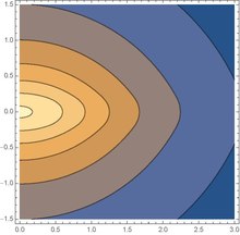
Note the somewhat pointed end of the equal potential in the (R,z) meridional plane of this R0=5z0=1 model

A unified thick disk potential

Consider an oblate potential in cylindrical coordinates

$${\begin{aligned}\Phi (R,z)&={GM_{0} \over 2z_{0}}\left[2\sinh ^{-1}\!\!Q-\sinh ^{-1}\!\!Q_{+}-\sinh ^{-1}\!\!Q_{-}\right]\\&={GM_{0} \over 2z_{0}}\log {({\sqrt {1+Q^{2}}}+Q)^{2} \over \left[{\sqrt {1+Q_{+}^{2}}}+Q_{+}\right]\left[{\sqrt {1+Q_{-}^{2}}}+Q_{-}\right]},\\Q_{\pm }&\equiv {R_{0}+\left|~|z|\pm z_{0}~\right| \over R},\\Q&\equiv {R_{0}+[0,|z|-z_{0}]_{\max } \over R},\\\end{aligned}}$$

where $z_{0},R_{0}$ are (positive) vertical and radial length scales. Despite its complexity, we can easily see some limiting properties of the model.

First we can see the total mass of the system is $M_{0}$ because

$$\Phi (R,z)\rightarrow {GM_{0} \over 2z_{0}}(2Q_{-}-Q_{-}-Q_{+})=-{GM_{0} \over R},$$

when we take the large radii limit $R\rightarrow \infty ,~|z|\geq z_{0},$, so that $Q=Q_{-}=Q_{+}-{2z_{0} \over R}={|z|+(R_{0}-z_{0}) \over R}\rightarrow 0.$

We can also show that some special cases of this unified potential become the potential of the Kuzmin razor-thin disk, that of the Point mass $M_{0}$, and that of a uniform-Needle mass distribution:

$$\Phi _{KM}(R,z)=-{GM_{0} \over {\sqrt {R^{2}+(|z|+R_{0})^{2}}}},~~z_{0}=0,$$

$$\Phi _{PT}(R,z)=-{GM_{0} \over {\sqrt {R^{2}+z^{2}}}},~~z_{0}=R_{0}=0,$$

$$\Phi _{UN}^{R_{0}=0}(R,z)={GM_{0} \over 2z_{0}}\left[2\sinh ^{-1}\!\!{(0,|z|-z_{0})_{\max } \over R}-\sinh ^{-1}\!\!{z_{0}+|z| \over R}-\sinh ^{-1}\!\!{\left|~z_{0}-|z|~\right| \over R}\right].$$

A worked example of gravity vector field in a thick disk

First consider the vertical gravity at the boundary,

$$g_{z}(R,z)=-\partial _{z}\Phi (R,z)=-{GM_{0}z \over 2z_{0}^{2}}\left[{1 \over {\sqrt {R_{0}^{2}+R^{2}}}}-{1 \over {\sqrt {(R_{0}+2z_{0})^{2}+R^{2}}}}\right],~~z=\pm z_{0},$$

Note that both the potential and the vertical gravity are continuous across the boundaries, hence no razor disk at the boundaries. Thanks to the fact that at the boundary, $\partial _{|z|}(2Q)-\partial _{|z|}Q_{-}=\partial _{|z|}\left(Q_{+}-{\frac {2z_{0}}{R}}\right)={1 \over R}$ is continuous. Apply Gauss's theorem by integrating the vertical force over the entire disk upper and lower boundaries, we have

$$2\int _{0}^{\infty }(2\pi RdR)|g_{z}(R,z_{0})|=4\pi GM_{0},$$

confirming that $M_{0}$ takes the meaning of the total disk mass.

The vertical gravity drops with

$$-g_{z}\rightarrow GM_{0}z(1+R_{0}/z_{0})/R^{3}$$

at large radii, which is enhanced over the vertical gravity of a point mass $GM_{0}z/R^{3}$ due to the self-gravity of the thick disk.

Density of a thick disk from Poisson Equation

Insert in the cylindrical Poisson eq.

$$\rho (R,z)={\partial _{z}\partial _{z}\Phi \over 4\pi G}+{\partial _{R}(R\partial _{R}\Phi ) \over 4\pi GR}={M_{0}R_{0}/z_{0} \over 4\pi (R^{2}+R_{0}^{2})^{3/2}}H(z_{0}-|z|),$$

which drops with radius, and is zero beyond $|z|>z_{0}$ and uniform along the z-direction within the boundary.

Note the vertically uniform thick disk density contour in this R0=5z0=1 model

Surface density and mass of a thick disk

Integrating over the entire thick disc of uniform thickness $2z_{0}$, we find the surface density and the total mass as

$$\Sigma (R)=(2z_{0})\rho (R,0),~~M_{0}=\int _{0}^{\infty }(2\pi RdR)\Sigma (R).$$

This confirms that the absence of extra razor thin discs at the boundaries. In the limit, $z_{0}\rightarrow 0$, this thick disc potential reduces to that of a razor-thin Kuzmin disk, for which we can verify ${|g_{z}(R,0+)| \over 2\pi G}\rightarrow \Sigma (R)\rightarrow {M_{0}R_{0} \over 2\pi (R^{2}+R_{0}^{2})^{3/2}}$.

Oscillation frequencies in a thick disk

To find the vertical and radial oscillation frequencies, we do a Taylor expansion of potential around the midplane.

$$\Phi (R_{1},z)\approx \Phi (R,0)+{\omega ^{2}R}(R_{1}-R)+{\kappa ^{2} \over 2}(R_{1}-R)^{2}+{\nu ^{2} \over 2}z^{2}$$

and we find the circular speed $V_{\text{cir}}$ and the vertical and radial epicycle frequencies to be given by

$$(R\omega )^{2}\equiv V_{\text{cir}}^{2}=\left[{(1+R_{0}/z_{0})GM_{0} \over {\sqrt {R^{2}+(R_{0}+z_{0})^{2}}}}-{(R_{0}/z_{0})GM_{0} \over {\sqrt {R^{2}+R_{0}^{2}}}}\right],$$

$$\nu ^{2}={GM_{0}(R_{0}/z_{0}+1) \over (R^{2}+(R_{0}+z_{0})^{2})^{3/2}},$$

$$\kappa ^{2}+\nu ^{2}-2\omega ^{2}=4\pi G\rho (R,0)={GM_{0}R_{0}/z_{0} \over (R^{2}+R_{0}^{2})^{3/2}}.$$

Interestingly the rotation curve $V_{\text{cir}}$ is solid-body-like near the centre $R\ll R_{0}$, and is Keplerian far away.

At large radii three frequencies satisfy ${\textstyle \left.\left[\omega ,\nu ,\kappa ,{\sqrt {4\pi G\rho }}\right]\right|_{R\to \infty }\to [1,1+R_{0}/z_{0},1,R_{0}/z_{0}]^{1 \over 2}{\sqrt {GM_{0} \over R^{3}}}}$. E.g., in the case that $R\to \infty$ and $R_{0}/z_{0}=3$, the oscillations $\omega :\nu :\kappa =1:2:1$ forms a resonance.

In the case that $R_{0}=0$, the density is zero everywhere except uniform needle between $|z|\leq z_{0}$ along the z-axis.

If we further require $z_{0}=0$, then we recover a well-known property for closed ellipse orbits in point mass potential,

$$\omega :\nu :\kappa =1:1:1.$$

A worked example for neutrinos in galaxies

For example, the phase space distribution function of non-relativistic neutrinos of mass m anywhere will not exceed the maximum value set by

$$f(\mathbf {x} ,\mathbf {v} ,t)={dN \over dx^{3}dv^{3}}\leq {6 \over (2\pi \hbar /m)^{3}},~~~$$

where the Fermi-Dirac statistics says there are at most 6 flavours of neutrinos within a volume $dx^{3}$ and a velocity volume

$$dv^{3}=(dp/m)^{3}=[(2\pi \hbar /dx)/m]^{3},$$

.

Let's approximate the distribution is at maximum, i.e.,

$$f(x,y,z,V_{x},V_{y},V_{z})={6 \over (2\pi \hbar /m)^{3}}q^{\alpha \over 2},~~0\leq q(E)={\Phi _{\max }-E \over V_{0}^{2}/2}\leq 1,$$

where $0\geq \Phi _{\max }\geq E=\Phi (x,y,z)+{V_{x}^{2}+V_{y}^{2}+V_{z}^{2} \over 2}\geq \Phi _{\min }\equiv \Phi _{\max }-{V_{0}^{2} \over 2}$ such that $E_{\min },E_{\max }$, respectively, is the potential energy of at the centre or the edge of the gravitational bound system. The corresponding neutrino mass density, assume spherical, would be

$$\rho (r)=n(x,y,z)m=\int dV_{x}\int dV_{y}\int dV_{z}~m~f(x,y,z,V_{x},V_{y},V_{z}),$$

which reduces to

$$\rho (r)={C(\Phi _{\max }-\Phi (r))^{3+\alpha \over 2} \over (\Phi _{\max }-\Phi _{\min })^{\alpha \over 2}},~~~C={6m\pi 2^{5/2}B\left(1+{\alpha \over 2},{3 \over 2}\right) \over (2\pi \hbar /m)^{3}}$$

Take the simple case $\alpha \to 0$, and estimate the density at the centre $r=0$ with an escape speed $V_{0}$, we have

$$\rho (r)\leq \rho (0)\rightarrow {m^{4}V_{0}^{3} \over \pi ^{2}\hbar ^{3}}\approx m_{\mathrm {eV} }^{4}V_{200}^{3}\times {\text{[Cosmic Critical Density]}}.$$

Clearly eV-scale neutrinos with $m_{eV}\sim 0.1-1$ is too light to make up the 100–10000 over-density in galaxies with escape velocity $V_{200}\equiv V/(\mathrm {200km/s} )\sim 0.1-3.4$, while neutrinos in clusters with $V\sim \mathrm {2000km/s}$ could make up $100-1000$ times cosmic background density.

By the way the freeze-out cosmic neutrinos in your room have a non-thermal random momentum ${\textstyle \sim {(\mathrm {2.7K} )k \over c}\sim (1~\mathrm {eV} /c^{2})(\mathrm {70km/s} )}$, and do not follow a Maxwell distribution, and are not in thermal equilibrium with the air molecules because of the extremely low cross-section of neutrino-baryon interactions.

A Recap on Harmonic Motions in Uniform Sphere Potential

Consider building a steady state model of the fore-mentioned uniform sphere of density $\rho _{0}$ and potential $\Phi (r)$

$${\begin{aligned}\rho (|\mathbf {r} |)&=\rho _{0}\equiv M_{\odot }n_{0},~~|\mathbf {r} |^{2}=x^{2}+y^{2}+z^{2}\leq r_{0}^{2},~~\Omega \equiv {\sqrt {4\pi G\rho _{0} \over 3}}\equiv {V_{0} \over r_{0}}\\\Phi (|\mathbf {r} |)&={\Omega ^{2}(x^{2}+y^{2}+z^{2})-3V_{0}^{2} \over 2}={V_{e}(r)^{2} \over 2}-\Phi (r_{0}),\end{aligned}}$$

where $V_{e}(r)=V_{0}{\sqrt {1-{r^{2} \over r_{0}^{2}}}}={\sqrt {2\Phi (r_{0})-2\Phi (r)}}$ is the speed to escape to the edge $r_{0}$.

First a recap on motion "inside" the uniform sphere potential. Inside this constant density core region, individual stars go on resonant harmonic oscillations of angular frequency $\Omega$ with

$${\begin{aligned}{\ddot {x}}=&-\Omega ^{2}x=-\partial _{x}\Phi ,\\{\ddot {y}}=&-\Omega ^{2}y,~~~{{\dot {y}}(t)^{2} \over 2}+{\Omega ^{2}y(t)^{2} \over 2}\equiv I_{y}(y,{\dot {y}})={{\dot {y}}(0)^{2} \over 2}+{\Omega ^{2}y(0)^{2} \over 2}\leq {(\Omega r_{0})^{2} \over 2}\\{\ddot {z}}=&-\Omega ^{2}z,\rightarrow {\dot {z}}(t)={\dot {z}}(0)\cos(\Omega t)+\Omega z(0)\sin(\Omega t).\end{aligned}}$$

Loosely speaking our goal is to put stars on a weighted distribution of orbits with various energies $f\left(I_{x}(x,{\dot {x}}),I_{y}(y,{\dot {y}}),I_{z}(z,{\dot {z}}\right)=DF(\mathbf {r} ,\mathbf {V} )$, i.e., the phase space density or distribution function, such that their overall stellar number density reproduces the constant core, hence their collective "steady-state" potential. Once this is reached, we call the system is a self-consistent equilibrium.

Example on Jeans theorem and CBE on Uniform Sphere Potential

Generally for a time-independent system, Jeans theorem predicts that $f(\mathbf {x} ,\mathbf {v} )$ is an implicit function of the position and velocity through a functional dependence on "constants of motion".

For the uniform sphere, a solution for the Boltzmann Equation, written in spherical coordinates $(r,\theta ,\phi )$ and its velocity components $(V_{r},V_{\theta },V_{\phi })$ is

$$f(r,\theta ,\varphi ,V_{r},V_{\theta },V_{\varphi })={C_{0} \over V_{0}^{3}}{\sqrt {V_{0}^{2} \over 2Q}},$$

where $C_{0}=2\pi ^{-2}\rho _{0}$ is a normalisation constant, which has the dimension of (mass) density. And we define a (positive enthalpy-like dimension ${\text{km}}^{2}/{\text{s}}^{2}$) Quantity

$$Q[\mathbf {x} ,\mathbf {v} ]\equiv \left[0,\left(-V_{0}^{2}-E\right)+{J^{2} \over 2r_{0}^{2}}\right]_{\max }.$$

Clearly anti-clockwise rotating stars with $J_{z}\leq 0,~~Q=0$ are excluded.

It is easy to see in spherical coordinates that

$J^{2}=r^{2}V_{t}^{2}=r^{2}(V_{\theta }^{2}+V_{\varphi }^{2}),$

$J_{z}=V_{\varphi }r\sin \theta ,$

$E={V_{r}^{2}+V_{t}^{2} \over 2}+\Phi (r),~V_{t}\equiv {\sqrt {V_{\theta }^{2}+V_{\varphi }^{2}}}$

Insert the potential and these definitions of the orbital energy E and angular momentum J and its z-component Jz along every stellar orbit, we have

$$2Q={\text{Heaviside}}\left({V_{\varphi } \over |V_{\varphi }|}\right)\times \left[V_{0}^{2}\left(1-{r^{2} \over r_{0}^{2}}\right)-V_{r}^{2}-\left(1-{r^{2} \over r_{0}^{2}}\right){\left(V_{\theta }^{2}+V_{\varphi }^{2}\right)},0\right]_{\max },$$

which implies $|V_{r}|\leq V_{e}(r)$, and $|V_{\theta }|,V_{\varphi }$ between zero and $V_{0}$.

To verify the above $E,~J_{z}$ being constants of motion in our spherical potential, we note

$$dE/dt={\partial E \over \partial t}+\mathbf {v} {\partial E \over \partial \mathbf {x} }+(\mathbf {-\nabla \Phi } ){\partial E \over \partial \mathbf {v} }$$

$$dE/dt={\partial \Phi \over \partial t}+\mathbf {v} {\partial \Phi \over \partial \mathbf {x} }+(\mathbf {-\nabla \Phi } )\mathbf {v} ={\partial \Phi \over \partial t}=0$$

for any "steady state" potential.

$$dJ_{z}/dt={\partial J_{z} \over \partial t}+{\partial J_{z} \over \partial \mathbf {x} }\cdot \mathbf {v} -(\mathbf {\nabla \Phi } )\cdot {\partial J_{z} \over \partial \mathbf {v} },$$

which reduces to $dJ_{z}/dt=0+[(V_{y})V_{x}+(-V_{x})V_{y}]-\left[(-y){x \over R}{\partial \Phi (R,z) \over \partial R}+(x){y \over R}{\partial \Phi (R,z) \over \partial R}\right]=0$ around the z-axis of any axisymmetric potential, where ${\textstyle R={\sqrt {x^{2}+y^{2}}}}$.

Likewise the x and y components of the angular momentum are also conserved for a spherical potential. Hence $dJ/dt=0$.

So for any time-independent spherical potential (including our uniform sphere model), the orbital energy E and angular momentum J and its z-component Jz along every stellar orbit satisfy

$$dE[\mathbf {x} ,\mathbf {v} ]/dt=dJ[\mathbf {x} ,\mathbf {v} ]/dt=dJ_{z}[\mathbf {x} ,\mathbf {v} ]/dt=0.$$

Hence using the chain rule, we have

$${d \over dt}Q(E[\mathbf {x} ,\mathbf {v} ],J[\mathbf {x} ,\mathbf {v} ],J_{z}[\mathbf {x} ,\mathbf {v} ])={\partial Q \over \partial E}{dE \over dt}+{\partial Q \over \partial J_{z}}{dJ_{z} \over dt}+{\partial Q \over \partial J}{dJ \over dt}=0,$$

i.e., ${\textstyle {d \over dt}f=f'(Q){dQ[\mathbf {x} ,\mathbf {v} ] \over dt}=0}$, so that CBE is satisfied, i.e., our

$$f(\mathbf {x} ,\mathbf {v} )=f(E[\mathbf {x} ,\mathbf {v} ],J[\mathbf {x} ,\mathbf {v} ],J_{z}[\mathbf {x} ,\mathbf {v} ])$$

is a solution to the Collisionless Boltzmann Equation for our static spherical potential.

A worked example on moments of distribution functions in a uniform spherical cluster

We can find out various moments of the above distribution function, reformatted as with the help of three Heaviside functions,

$$f(|\mathbf {r} |,V_{r},V_{\theta },V_{\varphi })={C_{0} \over 2V_{0}^{3}}\left.{\left(1-{|\mathbf {r} |^{2} \over r_{0}^{2}}\right)^{-1 \over 2}}\right.{(1-q)^{-1 \over 2}},~~q(\mathbf {r} ,\mathbf {V} )\equiv {V_{r}^{2} \over V_{e}(|\mathbf {r} |)^{2}}+{V_{\theta }^{2} \over V_{0}^{2}}+{V_{\varphi }^{2} \over V_{0}^{2}},$$

once we input the expression for the earlier potential $\Phi (r)$ inside $r\leq r_{0}$, or even better the speed to "escape from r to the edge" $r_{0}$ of a uniform sphere $V_{e}(r)=V_{0}{\sqrt {1-{r^{2} \over r_{0}^{2}}}}.$ Clearly the DF (distribution function) is well-defined only if $Q\geq 0\rightarrow q\leq 1$, which implies a narrow range on radius $0\leq |\mathbf {r} |<r_{0}$ and excludes high velocity particles, e.g., $V_{t}>V_{0}>V_{e}(r)$, from the distribution function (DF, i.e., phase space density).

In fact, the positivity carves an ellipsoid in the $[V_{r},V_{\theta },V_{\varphi }]$ velocity space ("velocity ellipsoid"),

$$q(\mathbf {r} ,\mathbf {V} )\equiv {V_{r}^{2} \over V_{0}^{2}(1-r^{2}/r_{0}^{2})}+\left({V_{\theta }^{2} \over V_{0}^{2}}+{V_{\varphi }^{2} \over V_{0}^{2}}\right)\equiv u_{r}^{2}+u_{\theta }^{2}+u_{\varphi }^{2}\leq 1,$$

where $(u_{r},u_{\theta },u_{\varphi })$ is $(V_{r},V_{\theta },V_{\varphi })$ rescaled by the function $V_{e}(r)=V_{0}{\sqrt {1-r^{2}/r_{0}^{2}}}$ or $V_{0}$ respectively.

The velocity ellipsoid (in this case) has rotational symmetry around the r axis or $V_{r}$ axis. It is more squashed (in this case) away from the radial direction, hence more tangentially anisotropic because everywhere $V_{e}(r)<V_{0}$, except at the origin, where the ellipsoid looks isotropic. Now we compute the moments of the phase space.

E.g., the resulting density (moment) is

$${\begin{aligned}\rho (r,\theta ,\varphi )&=\int _{-V_{e}(r)}^{V_{e}(r)}dV_{r}\int _{-V_{0}}^{V_{0}}dV_{\theta }\int _{0}^{V_{0}}dV_{\varphi }{C_{0} \over V_{0}^{3}}\left({2Q \over V_{0}^{2}}\right)^{-1/2}\\&=\int _{-1}^{1}\int _{-1}^{1}\int _{0}^{1}{(V_{e}du_{r})(V_{0}du_{\theta })(V_{0}du_{\varphi })C_{0} \over V_{0}^{3}(1-r^{2}/r_{0}^{2})^{1/2}(1-q)^{1/2}}\left.\right|_{q=u_{r}^{2}+u_{\theta }^{2}+u_{\varphi }^{2}}\\&=C_{0}{\int _{0}^{1}(1-u^{2})^{-1/2}(2\pi u^{2}du)}=\rho _{0}\end{aligned}}$$

is indeed a spherical (angle-independent) and uniform (radius-independent) density inside the edge, where the normalisation constant $C_{0}=2\pi ^{-2}\rho _{0}$.

The streaming velocity is computed as the weighted mean of the velocity vector

$${\begin{aligned}\langle \mathbf {V} \rangle (\mathbf {x} )&\equiv \\&={1 \over \rho }\int f(r,\theta ,\varphi ,V_{r},V_{\theta },V_{\varphi })d\mathbf {V} ^{3}[V_{r},V_{\theta },V_{\varphi }]\\&=\left[0,0,0\right],\end{aligned}}$$

thanks to the symmetry of $f(r,\theta ,\varphi ,V_{r},V_{\theta },V_{\varphi })=f(r,\theta ,\pm \varphi ,\pm V_{r},\pm V_{\theta },V_{\varphi })$, we have $\langle \mathbf {(\pm V_{r})V_{\varphi }} \rangle =0$, $~\langle \mathbf {(\pm V_{\theta })V_{\varphi }} \rangle =0$, $~\langle \mathbf {(\pm V_{r})V_{\theta }} \rangle =0$ everywhere}.

Likewise the rms velocity in the rotation direction is computed by a weighted mean as follows, E.g.,

$${\begin{aligned}\langle \mathbf {V} _{\varphi }^{2}\rangle (|\mathbf {x} |)&\equiv {\int fd\mathbf {V} ^{3}V_{\varphi }^{2} \over \rho (|\mathbf {r} |)}\\&={\int _{0}^{1}(2du_{r})\int _{0}^{\sqrt {1-u_{r}^{2}}}(2du_{\theta })\int _{0}^{\sqrt {1-u_{r}^{2}-u_{\theta }^{2}}}du_{\varphi }{(u_{\varphi }V_{0})^{2} \over (1-q)^{1/2}} \over \int _{0}^{1}{(2\pi u^{2}du)(1-u^{2})^{-1/2}}}\\&=0.25V_{0}^{2}=0.5\langle V_{t}^{2}\rangle \\&={\!\!\int _{0}^{1}(2du_{r})\!\!\int _{0}^{\sqrt {1-u_{r}^{2}}}(2du_{\varphi })\!\!\int _{0}^{\sqrt {1-u_{r}^{2}-u_{\varphi }^{2}}}du_{\theta }{(u_{\theta }V_{0})^{2} \over (1-q)^{1/2}} \over \int _{0}^{1}{(2\pi u^{2}du)(1-u^{2})^{-1/2}}}\\&=\langle \mathbf {V} _{\theta }^{2}\rangle (|\mathbf {x} |),\\\end{aligned}}$$

Here $\langle V_{t}^{2}\rangle =\langle V_{\theta }^{2}+V_{\varphi }^{2}\rangle =0.5V_{0}^{2}.$

Likewise

$$\langle \mathbf {V} _{r}^{2}\rangle (\mathbf {x} )={\!\!\int _{0}^{1}(du_{\varphi })\int _{0}^{\sqrt {1-u_{\varphi }^{2}}}\!\!(2du_{\theta })\!\!\int _{0}^{\sqrt {1-u_{\varphi }^{2}-u_{\theta }^{2}}}\!\!\!{(2du_{r})(u_{r}V_{e}(r))^{2} \over (1-q)^{1/2}} \over \int _{0}^{1}{(2\pi u^{2}du)(1-u^{2})^{-1/2}}}=\left({V_{0} \over 2}{\sqrt {1-{r^{2} \over r_{0}^{2}}}}\right)^{2}.$$

So the pressure tensor or dispersion tensor is

$${\begin{aligned}\sigma _{ij}^{2}(\mathbf {r} )=&{P_{ij}(\mathbf {r} ) \over \rho (\mathbf {r} )}\\=&\langle \mathbf {V} _{i}\mathbf {V} _{j}\rangle -\langle \mathbf {V} _{i}\rangle \langle \mathbf {V} _{j}\rangle \\=&{\begin{bmatrix}\left[1-({r \over r_{0}})^{2}\right]\left({V_{0} \over 2}\right)^{2}&0&0\\0&\left({V_{0} \over 2}\right)^{2}&0\\0&0&\left({V_{0} \over 2}\right)^{2}\end{bmatrix}}\end{aligned}}$$

with zero off-diagonal terms because of the symmetric velocity distribution.

The larger tangential kinetic energy than that of radial motion seen in the diagonal dispersions is often phrased by an anisotropy parameter

$$\beta (r)\equiv 1-{0.5\langle {\mathbf {V} _{t}}^{2}(|\mathbf {r} |)\rangle \over \langle {\mathbf {V} _{r}}^{2}\rangle (|\mathbf {r} |)}=1-{\langle {\mathbf {V} _{\theta }}^{2}(|\mathbf {r} |)\rangle \over \langle {\mathbf {V} _{r}}^{2}\rangle (|\mathbf {r} |)}=-{r^{2} \over r_{0}^{2}-r^{2}}\leq 0;$$

a positive anisotropy would have meant that radial motion dominated, and a negative anisotropy means that tangential motion dominates (as in this uniform sphere).

A worked example of Virial Theorem

Twice kinetic energy per unit mass of the above uniform sphere is

$${\begin{aligned}{2K \over M_{0}}&={\overline {\langle V^{2}\rangle }}\equiv \langle {\overline {V^{2}}}\rangle \\&=M_{0}^{-1}\int _{0}^{M_{0}}\langle V_{\theta }^{2}+V_{\varphi }^{2}+V_{r}^{2}\rangle dM\\&=M_{0}^{-1}\int _{0}^{1}\left({V_{0}^{2} \over 4}+{V_{0}^{2} \over 4}+{(1-x^{2})V_{0}^{2} \over 4}\right)d(x^{3}M_{0})=0.6V_{0}^{2},~~x\equiv {r \over r_{0}}=\left({M \over M_{0}}\right)^{1 \over 3}.\end{aligned}}$$

This balances the potential energy $-0.6V_{0}^{2}$ per unit mass of the uniform sphere, inside which $M\propto r^{3}\propto x^{3}$, because for this self-gravitating sphere, we can also verify that the virial per unit mass equals the averages of half of the potential

$${\begin{aligned}{E_{\text{pot}} \over M_{0}}&={\overline {\langle {\Phi \over 2}\rangle }}\\&=M_{0}^{-1}\int _{x>0}^{x<1}{\Phi (r_{0}x) \over 2}d(M_{0}x^{3})\\&={W \over M_{0}}={-2K \over M_{0}}.\end{aligned}}$$

Hence we have verified the validity of Virial Theorem for a uniform sphere under self-gravity, i.e., the gravity due to the mass density of the stars is also the gravity that stars move in self-consistently; no additional dark matter halo contributes to its potential, for example.

A worked example of Jeans Equation in a uniform sphere

Jeans Equation is a relation on how the pressure gradient of a system should be balancing the potential gradient for an equilibrium galaxy. In our uniform sphere, the potential gradient or gravity is

$$\nabla \Phi ={d\Phi \over dr}={\Omega ^{2}r}\geq 0,~~\Omega ={V_{0} \over r_{0}}.$$

The radial pressure gradient

$$-{d(\rho \sigma _{r}^{2}) \over \rho dr}=-{d\sigma _{r}^{2} \over dr}-{\sigma _{r}^{2} \over r}{d\log \rho \over d\log r}={\Omega ^{2}r \over 2}+0\geq 0.$$

The reason for the discrepancy is partly due to anisotropic pressure

$${\begin{aligned}{(\sigma _{\theta }^{2}-\sigma _{r}^{2}) \over r}&=0.25\Omega ^{2}r\geq 0\end{aligned}}$$

Now we can verify that (in absence of collisions)

$${\begin{aligned}{\partial \langle V_{r}\rangle \over \partial t}&=(-\sum _{i=x,y,z}V_{i}\partial _{i}\langle V_{r}\rangle )-\nabla _{r}\Phi +\sum _{i=x,y,z}{-\partial _{i}(n\sigma _{ir}^{2}) \over n}\\&={{\bar {V}}_{\theta }^{2}+{\bar {V}}_{\varphi }^{2}-2{\bar {V}}_{r}^{2} \over r}-{\partial \Phi \over \partial r}+\left[-{d(\rho \sigma _{r}^{2}) \over \rho dr}+{\sigma _{\theta }^{2}+\sigma _{\varphi }^{2}-2\sigma _{r}^{2} \over r}\right]\\&={0+0^{2}-2\times 0 \over r}-(\Omega ^{2}r)+\\&\left[{\Omega ^{2}r \over 2}+{(0.5V_{0})^{2}+(0.5V_{0})^{2}-2\times 0.25\Omega ^{2}(r_{0}^{2}-r^{2}) \over r}\right]\\&=0.\end{aligned}}$$

Here the 1st line above is essentially the Jeans equation in the r-direction, which reduces to the 2nd line, the Jeans equation in an anisotropic (aka $\beta \neq 0$) rotational (aka $\langle V_{\varphi }\rangle \neq 0$) axisymmetric ($\partial _{\varphi }\Phi (\mathbf {x} ,t)=0$ ) sphere (aka $\partial _{\theta }n(\mathbf {x} ,t)=0$) after much coordinate manipulations of the dispersion tensor; similar equation of motion can be obtained for the two tangential direction, e.g., ${\partial \langle V_{\varphi }\rangle \over \partial t}$, which are useful in modelling ocean currents on the rotating earth surface or angular momentum transfer in accretion disks, where the frictional term $-{\langle V_{\varphi }\rangle \over t_{\text{fric}}}$ is important.

The fact that the l.h.s. ${\partial V_{r} \over \partial t}=0$ means that the force is balanced on the r.h.s. for this uniform (aka $\nabla _{\mathbf {x} }mn(\mathbf {x} ,t)=0$) spherical model of a galaxy (cluster) to stay in a steady state (aka time-independent equilibrium ${\partial n(\mathbf {x} ,t) \over \partial t}=0$ everywhere) statically (aka with zero flow $\langle \mathbf {V} (\mathbf {x} ,t)\rangle =0$ everywhere). Note systems like accretion disk can have a steady net radial inflow $\langle \mathbf {V} (\mathbf {x} )\rangle <0$ everywhere at all time.

A worked example of Jeans equation in a thick disk

Consider again the thick disk potential in the above example. If the density is that of a gas fluid, then the pressure would be zero at the boundary $z=\pm z_{0}$. To find the peak of the pressure, we note that

$$P(R,z)=\int _{z}^{z_{0}}\partial _{z}\Phi \rho (R)dz=\rho (R)[\Phi (R,z_{0})-\Phi (R,z)].$$

So the fluid temperature per unit mass, i.e., the 1-dimensional velocity dispersion squared would be

$$\sigma ^{2}(R,z)={P(R,z) \over \rho (R)},~~|z|\leq z_{0}$$

$$\sigma ^{2}={GM_{0} \over 2z_{0}}\log {Q(z)Q(-z) \over Q(z_{0})Q(-z_{0})},~~Q(z)\equiv R_{0}+z_{0}+z+{\sqrt {R^{2}+(R_{0}+z_{0}+z)^{2}}}.$$

Along the rotational z-axis,

$$\sigma ^{2}(0,z)={GM_{0} \over 2z_{0}}\log {4(R_{0}+z_{0}+z)(R_{0}+z_{0}-z) \over 4R_{0}(R_{0}+2z_{0})}$$

$$\sigma (0,z)={\sqrt {GM_{0} \over 2z_{0}}}{\sqrt {\log {(R_{0}+z_{0})^{2}-z^{2} \over (R_{0}+z_{0})^{2}-z_{0}^{2}}}},$$

which is clearly the highest at the centre and zero at the boundaries $z=\pm z_{0}$. Both the pressure and the dispersion peak at the midplane $z=0$. In fact the hottest and densest point is the centre, where $P(0,0)={M_{0} \over 4\pi R_{0}^{2}z_{0}}{-GM_{0}\log[1-(1+R_{0}/z_{0})^{-2}] \over 2z_{0}}.$

A recap on worked examples on Jeans Eq., Virial and Phase space density

Having looking at the a few applications of Poisson Eq. and Phase space density and especially the Jeans equation, we can extract a general theme, again using the Spherical cow approach.

Jeans equation links gravity with pressure gradient, it is a generalisation of the Eq. of Motion for single particles. While Jeans equation can be solved in disk systems, the most user-friendly version of the Jeans eq. is the spherical anisotropic version for a static $\langle {v_{j}}\rangle =0$ frictionless system $t_{\text{fric}}\rightarrow \infty$, hence the local velocity spead $\sigma _{j}^{2}(r)=\langle {v_{j}^{2}}\rangle (r)-\underbrace {\langle {v_{j}}\rangle ^{2}(r)} _{=0}={\int \limits _{\infty }\!\!dv_{r}dv_{\theta }dv_{\varphi }({v}_{j}-\overbrace {\langle {v}\rangle _{j}^{p}} ^{=0})^{2}f_{p} \over \int \limits _{\infty }\!\!dv_{r}dv_{\theta }dv_{\varphi }f_{p}},$ everywhere for each of the three directions $~_{j}=~_{r},~_{\theta },~_{\varphi }$. One can project the phase space into these moments, which is easily if in a highly spherical system, which admits conservations of energy $E=$ and angular momentum J. The boundary of the system sets the integration range of the velocity bound in the system.

In summary, in the spherical Jeans eq.,

$${\begin{aligned}{d\Phi \over dr}=&{GM(r) \over r^{2}}\\=&-{d(n\langle {v_{r}^{2}}\rangle ) \over n(r)dr}+{\langle {v_{\theta }^{2}}\rangle +\langle {v_{\phi }^{2}}\rangle -2\langle {v_{r}^{2}}\rangle \over r},\\=&-{d(n\langle {v_{r}^{2}}\rangle ) \over n(r)dr},~~{\text{hydrostatic equilibrium if isotropic velocity }}\\=&{\langle v_{t}^{2}\rangle \over r},~~{\text{if purely centrifugal balancing of gravity with no radial motion}},\langle v_{t}^{2}\rangle \equiv \langle {v_{\theta }^{2}}\rangle +\langle {v_{\phi }^{2}}\rangle \end{aligned}}$$

which matches the expectation from the Virial theorem ${\overline {r\partial _{r}\Phi }}={\overline {v_{\text{cir}}^{2}}}={\overline {GM \over r}}={\overline {\langle v_{t}^{2}\rangle }}$, or in other words, the ${\overline {\text{global average}}}$ kinetic energy of an equilibrium equals the average kinetic energy on circular orbits with purely transverse motion.