The solution illustrated
edit
Essentially, the solution shown in orange,
(
r
^
rec
,
t
^
rec
)
{\displaystyle \scriptstyle ({\hat {\boldsymbol {r}}}_{\text{rec}},\,{\hat {t}}_{\text{rec}})}
, is the intersection of
light cones .
The
posterior distribution of the solution is derived from the product of the distribution of propagating spherical surfaces. (See
animation .)
Calculation steps
edit
A global-navigation-satellite-system (GNSS) receiver measures the apparent transmitting time,
t
~
i
{\displaystyle \displaystyle {\tilde {t}}_{i}}
satellites (
i
=
1
,
2
,
3
,
4
,
.
.
,
n
{\displaystyle \displaystyle i\;=\;1,\,2,\,3,\,4,\,..,\,n}
[1]
GNSS satellites broadcast the messages of satellites' ephemeris ,
r
i
(
t
)
{\displaystyle \displaystyle {\boldsymbol {r}}_{i}(t)}
δ
t
clock,sv
,
i
(
t
)
{\displaystyle \displaystyle \delta t_{{\text{clock,sv}},i}(t)}
[clarification needed as the functions of (atomic ) standard time , e.g., GPST .[2]
The transmitting time of GNSS satellite signals,
t
i
{\displaystyle \displaystyle t_{i}}
closed-form equations
t
~
i
=
t
i
+
δ
t
clock
,
i
(
t
i
)
{\displaystyle \displaystyle {\tilde {t}}_{i}\;=\;t_{i}\,+\,\delta t_{{\text{clock}},i}(t_{i})}
δ
t
clock
,
i
(
t
i
)
=
δ
t
clock,sv
,
i
(
t
i
)
+
δ
t
orbit-relativ
,
i
(
r
i
,
r
˙
i
)
{\displaystyle \displaystyle \delta t_{{\text{clock}},i}(t_{i})\;=\;\delta t_{{\text{clock,sv}},i}(t_{i})\,+\,\delta t_{{\text{orbit-relativ}},\,i}({\boldsymbol {r}}_{i},\,{\dot {\boldsymbol {r}}}_{i})}
δ
t
orbit-relativ
,
i
(
r
i
,
r
˙
i
)
{\displaystyle \displaystyle \delta t_{{\text{orbit-relativ}},i}({\boldsymbol {r}}_{i},\,{\dot {\boldsymbol {r}}}_{i})}
relativistic clock bias, periodically risen from the satellite's orbital eccentricity and Earth's gravity field .[2]
t
i
{\displaystyle \displaystyle t_{i}}
r
i
=
r
i
(
t
i
)
{\displaystyle \displaystyle {\boldsymbol {r}}_{i}\;=\;{\boldsymbol {r}}_{i}(t_{i})}
r
˙
i
=
r
˙
i
(
t
i
)
{\displaystyle \displaystyle {\dot {\boldsymbol {r}}}_{i}\;=\;{\dot {\boldsymbol {r}}}_{i}(t_{i})}
In the field of GNSS, "geometric range",
r
(
r
A
,
r
B
)
{\displaystyle \displaystyle r({\boldsymbol {r}}_{A},\,{\boldsymbol {r}}_{B})}
distance ,[3]
r
A
{\displaystyle \displaystyle {\boldsymbol {r}}_{A}}
r
B
{\displaystyle \displaystyle {\boldsymbol {r}}_{B}}
inertial frame (e.g., ECI one), not in rotating frame .[2]
The receiver's position,
r
rec
{\displaystyle \displaystyle {\boldsymbol {r}}_{\text{rec}}}
t
rec
{\displaystyle \displaystyle t_{\text{rec}}}
light-cone equation of
r
(
r
i
,
r
rec
)
/
c
+
(
t
i
−
t
rec
)
=
0
{\displaystyle \displaystyle r({\boldsymbol {r}}_{i},\,{\boldsymbol {r}}_{\text{rec}})/c\,+\,(t_{i}-t_{\text{rec}})\;=\;0}
inertial frame , where
c
{\displaystyle \displaystyle c}
speed of light . The signal time of flight from satellite to receiver is
−
(
t
i
−
t
rec
)
{\displaystyle \displaystyle -(t_{i}\,-\,t_{\text{rec}})}
The above is extended to the satellite-navigation positioning equation ,
r
(
r
i
,
r
rec
)
/
c
+
(
t
i
−
t
rec
)
+
δ
t
atmos
,
i
−
δ
t
meas-err
,
i
=
0
{\displaystyle \displaystyle r({\boldsymbol {r}}_{i},\,{\boldsymbol {r}}_{\text{rec}})/c\,+\,(t_{i}\,-\,t_{\text{rec}})\,+\,\delta t_{{\text{atmos}},i}\,-\,\delta t_{{\text{meas-err}},i}\;=\;0}
δ
t
atmos
,
i
{\displaystyle \displaystyle \delta t_{{\text{atmos}},i}}
atmospheric delay (= ionospheric delay + tropospheric delay ) along signal path and
δ
t
meas-err
,
i
{\displaystyle \displaystyle \delta t_{{\text{meas-err}},i}}
The Gauss–Newton method can be used to solve the nonlinear [disambiguation needed least-squares problem for the solution:
(
r
^
rec
,
t
^
rec
)
=
arg
min
ϕ
(
r
rec
,
t
rec
)
{\displaystyle \displaystyle ({\hat {\boldsymbol {r}}}_{\text{rec}},\,{\hat {t}}_{\text{rec}})\;=\;\arg \min \phi ({\boldsymbol {r}}_{\text{rec}},\,t_{\text{rec}})}
ϕ
(
r
rec
,
t
rec
)
=
∑
i
=
1
n
(
δ
t
meas-err
,
i
/
σ
δ
t
meas-err
,
i
)
2
{\displaystyle \displaystyle \phi ({\boldsymbol {r}}_{\text{rec}},\,t_{\text{rec}})\;=\;\sum _{i=1}^{n}(\delta t_{{\text{meas-err}},i}/\sigma _{\delta t_{{\text{meas-err}},i}})^{2}}
δ
t
meas-err
,
i
{\displaystyle \displaystyle \delta t_{{\text{meas-err}},i}}
r
rec
{\displaystyle \displaystyle {\boldsymbol {r}}_{\text{rec}}}
t
rec
{\displaystyle \displaystyle t_{\text{rec}}}
The posterior distribution of
r
rec
{\displaystyle \displaystyle {\boldsymbol {r}}_{\text{rec}}}
t
rec
{\displaystyle \displaystyle t_{\text{rec}}}
exp
(
−
1
2
ϕ
(
r
rec
,
t
rec
)
)
{\displaystyle \displaystyle \exp(-{\frac {1}{2}}\phi ({\boldsymbol {r}}_{\text{rec}},\,t_{\text{rec}}))}
mode is
(
r
^
rec
,
t
^
rec
)
{\displaystyle \displaystyle ({\hat {\boldsymbol {r}}}_{\text{rec}},\,{\hat {t}}_{\text{rec}})}
maximum a posteriori estimation .
The posterior distribution of
r
rec
{\displaystyle \displaystyle {\boldsymbol {r}}_{\text{rec}}}
∫
−
∞
∞
exp
(
−
1
2
ϕ
(
r
rec
,
t
rec
)
)
d
t
rec
{\displaystyle \displaystyle \int _{-\infty }^{\infty }\exp(-{\frac {1}{2}}\phi ({\boldsymbol {r}}_{\text{rec}},\,t_{\text{rec}}))\,dt_{\text{rec}}}
The GPS case
edit
{
Δ
t
i
(
t
i
,
E
i
)
≜
t
i
+
δ
t
clock
,
i
(
t
i
,
E
i
)
−
t
~
i
=
0
,
Δ
M
i
(
t
i
,
E
i
)
≜
M
i
(
t
i
)
−
(
E
i
−
e
i
sin
E
i
)
=
0
,
{\displaystyle \scriptstyle {\begin{cases}\scriptstyle \Delta t_{i}(t_{i},\,E_{i})\;\triangleq \;t_{i}\,+\,\delta t_{{\text{clock}},i}(t_{i},\,E_{i})\,-\,{\tilde {t}}_{i}\;=\;0,\\\scriptstyle \Delta M_{i}(t_{i},\,E_{i})\;\triangleq \;M_{i}(t_{i})\,-\,(E_{i}\,-\,e_{i}\sin E_{i})\;=\;0,\end{cases}}}
in which
E
i
{\displaystyle \scriptstyle E_{i}}
eccentric anomaly of satellite
i
{\displaystyle i}
M
i
{\displaystyle \scriptstyle M_{i}}
mean anomaly ,
e
i
{\displaystyle \scriptstyle e_{i}}
eccentricity , and
δ
t
clock
,
i
(
t
i
,
E
i
)
=
δ
t
clock,sv
,
i
(
t
i
)
+
δ
t
orbit-relativ
,
i
(
E
i
)
{\displaystyle \scriptstyle \delta t_{{\text{clock}},i}(t_{i},\,E_{i})\;=\;\delta t_{{\text{clock,sv}},i}(t_{i})\,+\,\delta t_{{\text{orbit-relativ}},i}(E_{i})}
The above can be solved by using the bivariate Newton–Raphson method on
t
i
{\displaystyle \scriptstyle t_{i}}
E
i
{\displaystyle \scriptstyle E_{i}}
inverse of Jacobian matrix as follows:
(
t
i
E
i
)
←
(
t
i
E
i
)
−
(
1
0
M
˙
i
(
t
i
)
1
−
e
i
cos
E
i
−
1
1
−
e
i
cos
E
i
)
(
Δ
t
i
Δ
M
i
)
{\displaystyle \scriptstyle {\begin{pmatrix}t_{i}\\E_{i}\\\end{pmatrix}}\leftarrow {\begin{pmatrix}t_{i}\\E_{i}\\\end{pmatrix}}-{\begin{pmatrix}1&&0\\{\frac {{\dot {M}}_{i}(t_{i})}{1-e_{i}\cos E_{i}}}&&-{\frac {1}{1-e_{i}\cos E_{i}}}\\\end{pmatrix}}{\begin{pmatrix}\Delta t_{i}\\\Delta M_{i}\\\end{pmatrix}}}
The GLONASS case
edit
The GLONASS ephemerides don't provide clock biases
δ
t
clock,sv
,
i
(
t
)
{\displaystyle \scriptstyle \delta t_{{\text{clock,sv}},i}(t)}
δ
t
clock
,
i
(
t
)
{\displaystyle \scriptstyle \delta t_{{\text{clock}},i}(t)}
See also
edit
In the field of GNSS,
r
~
i
=
−
c
(
t
~
i
−
t
~
rec
)
{\displaystyle \scriptstyle {\tilde {r}}_{i}\;=\;-c({\tilde {t}}_{i}\,-\,{\tilde {t}}_{\text{rec}})}
pseudorange , where
t
~
rec
{\displaystyle \scriptstyle {\tilde {t}}_{\text{rec}}}
δ
t
clock,rec
=
t
~
rec
−
t
rec
{\displaystyle \scriptstyle \delta t_{\text{clock,rec}}\;=\;{\tilde {t}}_{\text{rec}}\,-\,t_{\text{rec}}}
[1]
Standard GNSS receivers output
r
~
i
{\displaystyle \scriptstyle {\tilde {r}}_{i}}
t
~
rec
{\displaystyle \scriptstyle {\tilde {t}}_{\text{rec}}}
epoch .
The temporal variation in the relativistic clock bias of satellite is linear if its orbit is circular (and thus its velocity is uniform in inertial frame).
The signal time of flight from satellite to receiver is expressed as
−
(
t
i
−
t
rec
)
=
r
~
i
/
c
+
δ
t
clock
,
i
−
δ
t
clock,rec
{\displaystyle \scriptstyle -(t_{i}-t_{\text{rec}})\;=\;{\tilde {r}}_{i}/c\,+\,\delta t_{{\text{clock}},i}\,-\,\delta t_{\text{clock,rec}}}
round-off-error resistive during calculation.
The geometric range is calculated as
r
(
r
i
,
r
rec
)
=
|
Ω
E
(
t
i
−
t
rec
)
r
i
,
ECEF
−
r
rec,ECEF
|
{\displaystyle \scriptstyle r({\boldsymbol {r}}_{i},\,{\boldsymbol {r}}_{\text{rec}})\;=\;|\Omega _{\text{E}}(t_{i}\,-\,t_{\text{rec}}){\boldsymbol {r}}_{i,{\text{ECEF}}}\,-\,{\boldsymbol {r}}_{\text{rec,ECEF}}|}
Earth-centred, Earth-fixed (ECEF) rotating frame (e.g., WGS84 or ITRF ) is used in the right side and
Ω
E
{\displaystyle \scriptstyle \Omega _{\text{E}}}
transit time .[2]
Ω
E
(
t
i
−
t
rec
)
=
Ω
E
(
δ
t
clock,rec
)
Ω
E
(
−
r
~
i
/
c
−
δ
t
clock
,
i
)
{\displaystyle \scriptstyle \Omega _{\text{E}}(t_{i}\,-\,t_{\text{rec}})\;=\;\Omega _{\text{E}}(\delta t_{\text{clock,rec}})\Omega _{\text{E}}(-{\tilde {r}}_{i}/c\,-\,\delta t_{{\text{clock}},i})}
The line-of-sight unit vector of satellite observed at
r
rec,ECEF
{\displaystyle \scriptstyle {\boldsymbol {r}}_{\text{rec,ECEF}}}
e
i
,
rec,ECEF
=
−
∂
r
(
r
i
,
r
rec
)
∂
r
rec,ECEF
{\displaystyle \scriptstyle {\boldsymbol {e}}_{i,{\text{rec,ECEF}}}\;=\;-{\frac {\partial r({\boldsymbol {r}}_{i},\,{\boldsymbol {r}}_{\text{rec}})}{\partial {\boldsymbol {r}}_{\text{rec,ECEF}}}}}
The satellite-navigation positioning equation may be expressed by using the variables
r
rec,ECEF
{\displaystyle \scriptstyle {\boldsymbol {r}}_{\text{rec,ECEF}}}
δ
t
clock,rec
{\displaystyle \scriptstyle \delta t_{\text{clock,rec}}}
The nonlinearity of the vertical dependency of tropospheric delay degrades the convergence efficiency in the Gauss–Newton iterations in step 7.
The above notation is different from that in the Wikipedia articles, 'Position calculation introduction' and 'Position calculation advanced', of Global Positioning System (GPS). See also
edit
References
edit
^ a b Misra, P. and Enge, P., Global Positioning System: Signals, Measurements, and Performance, 2nd, Ganga-Jamuna Press, 2006.
^ a b c d e f The interface specification of NAVSTAR GLOBAL POSITIONING SYSTEM ^ 3-dimensional distance is given by
r
(
r
A
,
r
B
)
=
|
r
A
−
r
B
|
=
(
x
A
−
x
B
)
2
+
(
y
A
−
y
B
)
2
+
(
z
A
−
z
B
)
2
{\displaystyle \displaystyle r({\boldsymbol {r}}_{A},\,{\boldsymbol {r}}_{B})=|{\boldsymbol {r}}_{A}-{\boldsymbol {r}}_{B}|={\sqrt {(x_{A}-x_{B})^{2}+(y_{A}-y_{B})^{2}+(z_{A}-z_{B})^{2}}}}
r
A
=
(
x
A
,
y
A
,
z
A
)
{\displaystyle \displaystyle {\boldsymbol {r}}_{A}=(x_{A},y_{A},z_{A})}
r
B
=
(
x
B
,
y
B
,
z
B
)
{\displaystyle \displaystyle {\boldsymbol {r}}_{B}=(x_{B},y_{B},z_{B})}
inertial frame .
External links
edit
PVT (Position, Velocity, Time): Calculation procedure in the open-source GNSS-SDR and the underlying RTKLIB 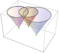 Essentially, the solution shown in orange, , is the intersection of light cones.
 The posterior distribution of the solution is derived from the product of the distribution of propagating spherical surfaces. (See animation.)


